Sheng Hao was born in Lanzhou He received his B E and M S degrees in computer science and technology from Wuhan University He is now a Ph D candidate of architecture His research interests include wireless network, communication theory and complex network theory
, E-mail:2008301500139@whu.edu.cn.
Huyin Zhang was born in Shanghai He received his Ph D degree in computer science and technology from Wuhan university He is a professor of Wuhan university His research interests include high performance computing, network quality of service, new generation network architecture
, E-mail:zhy2536@whu.edu.cn.
Mengkai Song was born in Wuhan He received his undergraduate degree in computer science and technology from Wuhan university He is now a graduate student of computer network His research interests include wireless network and differential privacy
, E-mail:mksong@whu.edu.cn.
Abstract
The mobile Ad Hoc network (MANET) is a self-organizing and self-configuring wireless network, consisting of a set of mobile nodes. The design of efficient routing protocols for MANET has always been an active area of research. In existing routing algorithms, however, the current work does not scale well enough to ensure route stability when the mobility and distribution of nodes vary with time. In addition, each node in MANET has only limited initial energy, so energy conservation and balance must be taken into account. An efficient routing algorithm should not only be stable but also energy saving and balanced, within the dynamic network environment. To address the above problems, we propose a stable and energy-efficient routing algorithm, based on learning automata (LA) theory for MANET. First, we construct a new node stability measurement model and define an effective energy ratio function. On that basis, we give the node a weighted value, which is used as the iteration parameter for LA. Next, we construct an LA theory-based feedback mechanism for the MANET environment to optimize the selection of available routes and to prove the convergence of our algorithm. The experiments show that our proposed LA-based routing algorithm for MANET achieved the best performance in route survival time, energy consumption, energy balance, and acceptable performance in end-to-end delay and packet delivery ratio.
Keywords:MANET routing
;
stability measurement model
;
effective energy ratio function
;
learning automata theory
;
feedback mechanism
;
optimization
Sheng Hao. A Stable and Energy-Efficient Routing Algorithm Based on Learning Automata Theory for MANET. [J], 2018, 3(2): 43-57 doi:10.1007/s41650-018-0012-7
Ⅰ. INTRODUCTION
The mobile Ad Hoc network(MANET)is composed of aset of self-wireless mobile nodes, communicating with out a fixed communication network infrastructure[1,2,3,4,5]. Owing to its flexible and dynamic nature, MANET has been widely used in areas such as military communications, disaster area communications, and emergency rescues. MANET has also been used to ensure vehicle communication by constructing vehicular Ad Hoc network(VANET). To enhance communication quality, MANET needs efficient routing protocols. In this network, each node has stochastic mobility and distribution, causing the network topology to vary with time. It is therefore difficult to ensure the stability of selected routes. Considering the limited initial energy of each node, it is important to reduce energy consumption and also to balance residual energy. To date, many MANET routing algorithms have been proposed to enhance communication performance.
A. Motivation
Although a large amount of meaningful work has been conducted on the design of MANET routing, none of this work considers the impact of node distribution, which varies over time and affects route stability. Work that focuses on enhancing the stability of routing topology and using mobility prediction models (e. g. , Refs. [6,7,8,9,10,11,12,13,14,15])may therefore not fully consider mobility control. In addition, most existing MANET routing algorithms use traditional heuristic algorithms as their optimization methods(e. g. , Refs. [16,17,18,19,20,21,22]); these may lack expansibility and offer minimal hand-tuning, resulting in relatively high computation costs in a dynamic environment. From the engineering application point of view, MANET has been widely used in many infrastructure and emergency communication applications. The new generation version of MANET can use non-orthogonal multiple access technique, which greatly enhances its performance. The existing problems and practical value discussed above motivated us to design a stable and energy-efficient routing algorithm for MANET.
B. Contributions
The major contributions of this paper can be summarized as follows.
1)We construct a new stability measurement model to measure the relay node stability in a route and define an effective energy ratio function.
2)We introduce the learning automata(LA)theory to optimize the process of route selection.
3)We construct a MANET environment feedback mechanism using LA theory. With the help of this MANET environment feedback mechanism, we can choose the optimal path from the source node to the destination node. This will be more stable, ensuring energy conservation and balance.
4)We provide a rigorous and skillful mathematical proof to authenticate the algorithm’s convergence, which has not been done successfully in previous work.
C. Paper Outline
The rest of our paper is organized as follows. The related work of the MANET routing algorithm is reviewed in section Ⅱ. A brief overview of the routing protocol and LA is presented in section Ⅲ. The system model is presented in section Ⅳ. The proof of convergence is provided in section V. The simulation results and experiment analysis are presented in section Ⅵ. Finally, a conclusion summarizes these findings in section Ⅶ.
Ⅱ. RELATED WORK AND OUR SOLUTION
To the best of our knowledge, most current routing algorithms proposed for MANET focus mainly on enhancing routing stability (e. g. , Refs. [6,7,8,9,10,11,12,13] . Typically, in Ref. [7], B. An et al. proposed a mobility-based hybrid routing protocol. By dividing the network into several dynamic and adaptive teams, the mobility behavior of each team can be predicted by constructing a team mobility model. A hybrid routing protocol is then proposed for team communication. However, in a practical network environment, each node has independent stochastic mobility; a team mobility model cannot reflect the changes in a team. If the relative mobility of nodes in a team is high enough, the accuracy of this model must be reduced. In Ref. [8], A. Bentaleb et al. proposed a new mobility model, based on the Doppler shift, which can estimate relative speed. Using this mobility model enables the design of a mobility-based clustering routing protocol. Although this method ensures that the selected route has relatively high stability, the nodes must periodically exchange HELLO packets with neighbor nodes, which, of course, increases the energy consumption of the nodes. In Ref. [11], R. Suraj et al. used movement history and genetic policy to construct a direction prediction adjacency matrix. This technique proposes a new approach to mobility prediction, which does not depend on probabilistic methods and is completely based on a genetic algorithm(GA). However, it must be noted that this method cannot ensure normalization; it also incurs relatively high computation costs(owing to the prediction adjacency matrix). In Ref. [12], T. Manimegalai et al. proposed an animal communication strategy(ACS), based on a routing algorithm. By using ACS, the authors constructed an animal behavior mechanism to improve path construction and retention, enhancing route stability. This method is similar to the ant colony algorithm, which uses history information to adjust the relay nodes. In this method, the authors declared that the density of the node is very important for enhancing route topology and communication stability. This rule is modeled on the gregarious habits of animals. Therefore, a node that has a relatively high node density is chosen as the relay node. The adjustment mechanism for the relay node also follows this rule. It should be stressed that, in this method, the source node needs to periodically send a request packet to the destination node.
In addition, many routing algorithms focus on improving other qualities (e. g. , Refs. [16,17,18,19,20,21,22]), including energy consumption, end-to-end delay, and the packet delivery ratio. In a typical example[17], S. Chettibi et al. proposed an adaptive maximum-lifetime routing policy based on reinforcement learning strategy. With the help of the heuristic principle(Qlearning method), it optimizes the route lifetime and minimizes overhead control. In this method, the author constructs an intelligence battery model, which can help the node adjust its transmission power, based on the dynamic environment. In Ref. [18], a network routing protocol is proposed, based on the Russian Doll method. In this method, the routing protocol can choose the best multi-criteria solution to reduce energy consumption and enhance the throughput ratio. In Ref. [19], S. Chettibi et al. proposed a routing algorithm based on the ant colony optimization technique. By using the ant colony algorithm, the authors constructed an estimate model to represent route preference. In this method, the battery equipped with a node is sufficiently intelligent to adjust its battery loss rate. The heuristic strategy proposed in this paper relies on this precondition, which may not fit all MANETs. Ref. [20]proposed to select a stable route by using a fuzzy logic system. In Ref. [21], P. Srivastava et al. achieved a QoS-aware routing by using an artificial neural network (ANN). This approach used a convolution calculation to achieve good performance in routing QoS(in this algorithm, the optimization targets are the packet delivery ratio and end-to-end delay; for this reason, the parameters needed in cable news network(CNN)are a packet delivery ratio and end-to-end delay. It is worth noting that the convolution calculation model constructed in this paper can raise computation costs(in this paper, as the authors have used a two-layer CNN, the measurement parameters have had to be computed multiple times). In addition, as a general rule, the computation accuracy and time of CNN always depend on the number of layers.
We point out the advantages and disadvantages of each routing algorithm[6,22]. It should be noted that none of the works mentioned considers the impact of node distribution, which varies with time and also affects route topology stability(the route life cycle). In fact, the survival time of a route is influenced by not only the relative mobility between nodes but also the distribution of nodes. Overall energy conservation and balance should also be taken into consideration. In addition to the above two points, it must be stressed that the traditional heuristic techniques and machine learning methods used to design MANET routing protocols generally lack expansibility. They have minimal hand-tuning, and incur relatively high computation costs. To resolve these existing problems, this paper proposes a stable and energy-efficient routing algorithm for MANET using LA theory. Compared with traditional machine learning methods and heuristic algorithms, LA theory has the following advantages: (1)LA theory is supported by a completed mathematics proof[23,24,25,26]; (2)LA theory is capable of global optimization and results in relatively low costs, in a dynamic environment; (3)LA theory has good expansibility, which is needed to optimize large-scale MANET routing performance; (4) LA theory can map the computation space to a probability space, ensuring normalization. The optimization efficiency of traditional heuristic algorithms and machine learning methods(e. g. , ACO, PSO, GA)rely on the construction of a heuristic function. Considering the dynamic environment, it is difficult to construct a good enough heuristic function. In addition, these methods cannot always ensure normalization. As a general rule, the LA theory is used in bio-computation and stochastic system control, which can be regarded as a dynamic environment. Owing to the dynamic features of MANET, we are able to use LA theory to find the optimal route from available paths.
In our solution, we begin by constructing a new node stability measurement model and defining the effective energy ratio function. On this basis, we introduce a node-weighted value function, which is used as the iteration parameter. We then use LA theory to construct a MANET environment feedback model. In this feedback model, each node is equipped with learning automaton, enabling it to take action by sensing the surrounding environment. Based on LA theory, this process can be represented through a rigorous linear probability iteration; in other words, the relay node in the available paths updates its weighted value according to the feedback signal, which represents the result after sensing the environment(we have used a judging function to distinguish the type of feedback signal explained in part A of section Ⅳ). When the feedback signal is a reward signal, this node will add its weighted value. Conversely, it will reduce its weighted value. Thus, the current node can decide which node should be chosen as the next hop node from a group of available hop nodes. Accordingly, the path value defined in this feedback mechanism will be added or reduced(before executing this mechanism, we found all available paths from the source node to the destination node explained in part A of section Ⅳ). Because of the convergence of LA, we can finally choose the optimal path with the highest path value from all of the available paths. The chosen path will be stable enough to ensure overall energy saving and balance.
Ⅲ. PRELIMINARIES AND BACKGROUND
In this section, we present a brief overview of routing protocols and some preliminary information on LA theory.
A. Overview of Routing Protocols
Based on the relation with information[20,27], routing protocols can be divided into several categories. In general, we classify the protocols into three kinds: proactive, reactive and hybrid protocols. Proactive routing protocols periodically update the message so that it can ensure the data packets transmission. Reactive protocols initiate route discovery on demand. That means when the source node has data packets to be sent to a given destination node, it initiates route discovery by broadcasting the route request packet. While receiving the request packet, the relay nodes will rebroadcast it again. This process continues until the request packet arrives at the destination node. Similar to the handshake mechanism, the destination node generates a route reply packet and sends it to the source node. In other words, the reply packet tracks the reverse route already taken by the corresponding request packet. As a compromised scheme, hybrid routing protocols combine these two routing protocols, which can be used in hierarchical structure networks. Generally, proactive protocols cause more energy consumption, which, of course, degrades the network life cycle. Hybrid routing protocols use more control information than reactive protocols needing a hierarchical structure network.
B. Learning Automata
LA theory is a self-learning mechanism based on the theory of stochastic process[23,26]. As an adaptive decision-making system, LA can enhance the performance by using previous knowledge to choose the best action from a limited set of actions through repeated interactions with a random environment. Basic LA contains three key factors: a random environment, an automaton and a feedback system. The automaton chooses actions based on the random environment and the environment responds to these actions by producing a feedback signal. Based on the effect on the automaton, the feedback signal can be divided into‘positive signal’(reward signal)or‘negative’signal(penalty signal). Over a period of time, the automaton can learn from the feedback signal to find an optimal action(Fig.1 shows the operating principle of LA).
(environment) The random environment is an object interacting with the automaton. Usually, we set E ={A, B, C} to describe the random environment. Where A={α1, α2, …, αt}represents the limited sets of inputs performed by the automaton, αt represents the action in time slot t. Similarly, B={β1, β2, …, βt} represents a limited set of responses from the random environment, βt represents the response from the environment in time slot t. C={c1, c2, …, ct}is the set of penalty probabilities, which is associated with the given action α in time slot t.
Using the definition of ci, the average penalty M(t)can be defined by the following expression:
M(t)=E[β(t)|P(t)]
=E[β(t)|p1(t), p2(t), …, pn(t)]
=Pr[β(t=0)|P(t)]
=
=,
where P(t)represents the action probability at instant t. Thus, the average penalty for the pure chance automaton is expressed as
(automaton) In a general sense, an automaton is a work system which does not need guidance from the outside. From the mathematical point of view, the automaton can be defined as{A, B, Q, T, G}(A=α1, α2, …, αt, B=β1, β2, …, βt have been defined in Definition 1). Q=q1(t), q2(t), …, qn(t)represents the state in time slot t. T : Q×B×A−→Q denotes the state transition function of the automaton, which determines the way in which automaton transfers to the next state from the current state and input. We usually use the following formula to represent the state transition from instant t to t+1.
G determines the output based on the state at instant t.
Ⅳ. SYSTEM MODEL
In this section, we construct a new stability measurement model and define an effective energy ratio function. On this basis, we define the node-weighted value function, which can be used to construct a MANET environment feedback mechanism(a routing learning process).
A. Network Model
In general, a MANET can be described by a undirected graph G=(V, E), where V represents the set of nodes and E represents the set of edges[28,29]. Therefore, a path in the network can be regarded as a set of nodes, which connect to each other from the source node to the destination node. In our paper, all nodes exist in a 2D rectangular scenario and communicate through a common broadcast channel using omnidirectional antennas. They have the same transmission range of r. Assuming that the distance between node i and j can be represented as Dist(i, j)and j is i’s neighbor node, Dist(i, j) should be no more than r. Additionally, we do not have to consider the impact of an interference range or avoid collision by using a shared wireless channel. It should be explained that these preconditions have been widely adopted in previous work.
B. Node Stability Measurement Model
The chosen relay node in an available path from the source node to the destination node should be stable enough to ensure path stability. This distinguishes our work from previous studies, in which we used only node velocity and did not consider the impact of the distribution of neighbor nodes on stability. We measure the node stability by estimating the average time a node is connected to its neighbor nodes. Without any loss of generality, we assume that vi represents the mobility speed of node i in a small time slot, and that the velocity of the node remains unchanged during this short period of time. Hence, we can estimate the survival time of the link between node i and any of its neighbor nodes, using the following formula:
where , represent the horizontal component and ver-tical component of speed, respectively; Dist()x, Dist()y the horizontal component and vertical component of the current distance between node i and node j; node j is a neighbor node of node i. By solving the above formula, we can get the ex-pression of ti, j
where Ha, Hb, Hc can be represented as
Thus, we can use a weighted average function to measure node i’s stability(Nsi)
where π{current distance = Dist(i, j)} represents the weighted value of ti j, which means the limiting probability that the current distance between i and j is Dist(i, j). To give the expression of π{current distance=Dist(i, j)}, we should first deduce the expression of Prob{Dist(i, j)< r}(r is the transmission range defined in part A of section Ⅲ).
Without loss of generality, the node mobility in this MANET is independent and stochastic. Thus, we can deduce the spatial PDF(probability distribution function)of any node in the MANET using the following uniform distribution:
where L, W respectively represent the length and width of MANET. Therefore, the joint PDF between node i and j can be represented as follows, noting that the joint PDF relies on the setting of network scenarios
Thus, the expression of Prob{Dist(i, j)6 r} can be expressed as
Simplifying the above integral (7) using the elementintegral method
where funit(D)can be written as
Generally, the transmission range r is always less than the width W. With the help of the spline interpolation method[30,31], we can deduce the expression of π{current distance=Dist(i, j)}
D is a simplified representation of Dist() in previous formulas. The reason we get the expression (10) through the spline interpolation method is that it meets Lip-schitz Condition[30,32].
By substituting formula(10)into formula(4), we can obtain Ns.
C. Effective Energy Ratio Function
In an available path, the chosen relay node should have enough power to ensure the transmission of packets. We use the effective energy ratio function(Er)to represent the energy level of the relay node
where Rei and Iei represent the residual energy and initial energy of node i, respectively. Thus, we can define the node weighted value(Nw)as
where ω()represents the weighting factor, Nb0i represents the normalized value of Nbi. To find the optimal route among all of the available routes, ensuring that it is not only stable but also guarantees energy conservation and balance, it is necessary to optimize the selection of paths. We note that traditional heuristic routing algorithms generally lack extendibility, mathematical rigor, and adaptability for a dynamic environment. Therefore, unlike previous work, we have chosen LA theory to complete the optimization process. In the next section, we discuss in more detail our LA theory-based, energy-efficient, stable routing algorithm.
Ⅴ. STABLE AND ENERGY EFFICIENT ROUTING ALGORITHM BASED ON LA THEORY
In this section, we first use LA theory to construct a MANET environment feedback mechanism. In other words, by judging the content of each reply message, we reward or punish the relay node through a rigorous iteration expression. We then provide a detailed algorithm implementation scheme. Finally, we prove the convergence of our algorithm.
A. MANET Environment Feedback Mechanism
When the source node plans to send packets to the destination node, it needs to find the available paths from the source node to destination node. To find all of the available paths to the destination node, the source node broadcasts build-route messages to its neighbor nodes(flooding requests). Once the build-route message is received by the destination node, it will reply the build-route message, so that all available paths from the source node to the destination node can be identified. Obviously, not all of these paths will be good enough to transmit data packets. Therefore, it is necessary to find the optimal path, which is sufficiently stable and ensures overall energy saving and balance.
Using LA theory, we construct a MANET environment feedback model, which is an optimization mechanism for route selection. In this model, each node is equipped with a learning automaton to execute the feedback mechanism. Fig.2 shows the feedback mechanism of the LA. To find the optimal path from the available paths, the source node sends request packets to the destination node through the available paths. When it receives the request packets, the destination node responds by sending reply packets to the source node along the available paths. In this reply process, each relay node on an available path receives a reply packet from the next available hop node. Drawing on LA theory, the next available hop node senses the surrounding MANET environment and adds environment-feedback information to the reply message.
As mentioned in section Ⅱ, there are two types of environment feedback. Based on the information content of the replies, we set two feedback criteria(Fig.3 shows these two criteria, where j and k represent the next available hop nodes of node i):
(1) If a relay node receives a reply packet from the next hop node, and the information contained in this reply packet is“good information”(a reward signal), we will execute the reward scheme and the weighted value(Nw)of the next hop node will be increased accordingly.
(2)If a relay node receives the reply packet from its next hop node, and the information contained in this reply packet is“bad information”(a penalty signal), we will execute penalty scheme and the weighted value(Nw)of the next hop node will be reduced accordingly.
Using the standard linear iteration equation of LA theory[23], the node’s reward feedback scheme for receiving“good information”can be represented as
The penalty feedback scheme for altering a node’s weighted value on receipt of“bad information”can be represented as
where a and b represent the linear update rate of the weighted value; t represents the instant(in a discrete condition, it denotes iteration times).
It is now essential to define a feedback judgement function, which can decide whether information is good or bad. Based on the definition of feedback judgement function in LA theory[23], the feedback judgment function(ϕ)can be expressed as
where Ni represents the number of node i’s neighbor nodes. When Nwi(t)> 0(better than the average level), the MANET environment has generated a reward feedback signal and the node has received good information; conversely, Nwi(t)< 0 (worse than the average level)means that the MANET environment has generated a penalty feedback signal and the node has received bad information.
We note that only using formulas(13)and(14)cannot reflect feedback strength, as they change with iteration times. Therefore, we continue to optimize these two formulas, using the following expression to represent the improved feedback scheme:
where
As the node-weighted value updates, based on our proposed MANET feedback mechanism, the path-weighted value will be updated accordingly. In this feedback mechanism, the path value(P)of an available path from the source node to the destination node can be represented as
where M represents the number of relay nodes on an available path from the source node to the destination node; m represents the ID of the available path. With the help of this feedback mechanism, the node learns from the information by sensing the MANET environment(judging the type of feedback signal) and updates its weighted value. With the help of this feedback mechanism, we can find the optimal path, with the highest path value P. Finally, the data packets will be transmitted through this optimal path that is stable enough and ensures overall energy conservation and balance.
B. Algorithm Implementation Scheme
We give the detailed algorithm implementation scheme as follows:
C. Convergence Proof of Our Proposed Routing Algorithm
As mentioned in a previous paper, our proposed algorithm uses LA theory to optimize the selected paths. As it is important to ensure the convergence of this process, we have provided the following rigorous proof.
Our proposed routing algorithm
Initialization:
adjustable parameters of LA(δ, ε)
Input:
the available paths between the source node and the destination node(α. ), relay nodes which belong to the available paths
Output:
the optimal path
Execution steps:
1)sending a packet through an available path;
2)while receiving the packet, the destination node will send a reply message to the source node;
3)for i=1, 2, ···, m−1(i represents the relay node ID);
4)if the relay node i receives a reply message from the next available hop node j and ;
5)using the reward feedback scheme to update the weighted value of node j;
6)Nwj(t+1)=Nwj(t)+aj(t)[1−Nwj(t)];
7)updating the path value which contains this relay node j accordingly;
8)Pm(t+1)=Pm(t)+(aj(t)[1−Nwj(t)])/M;
9)else(node i receives the reply message from the available next hop node j and = ;
10) using the penalty feedback scheme and updating the weighted value of the node j;
11)Pj(t+1)=[1−bj(t)]pj(t);
12)updating the path value which contains this relay node j accordingly;
13)Pm(t+1)=Pm(t)+[bj(t)]/M;
End
The node-weighted value Nw(t)can converge if and only if the drift of the node-weighted value Nw0(t)is not a direct function of the instant t.
the drift of node weighted value Nw0(t) is not directly a function of instant t.
As the process of this algorithm can be regarded as an optimization problem, we can use approximation theory[32]to prove the algorithm. In our paper, each node has a learning automaton; for this reason, we can use the theory of stochastic process to represent the genericity update process of weighted value(in the dynamics control method, the one step probability update is called the drift function of probability because the long update process can be regarded as a continuous update process. For this reason, we can present the genericity update process of node-weighted value in this way:
Based on the Kolmogorov criterion[23], formula(19)can be represented as
Based on the definition in LA theory, Λ represents the genericity maximum update rate proposed in our improved LA. Generally, the update rate floats around 0.10(in our paper, we set δ =0.10 and ε=0.10). Thus, we can reach the following conclusion by differentiating both sides of the formula(20)
Let , can be represented as
Obviously, we conclude that is not a direct function of the time slot t. This conclusion allows us to use the spline interpolation method[31] to rewrite the node-weighted value Nw(t)
where τ∈[nΛ, (n+1)Λ], PΛ(τ)is a piecewise constant interpolation function(In LA theory, P(t)represents the action probability at instant t). Now we only care about the convergence of PΛ().
Generally, the genericity maximum update rate Λ is close to 0[23]. Hence, based on approximation theory[33], we can make an assertion that pΛ(τ)can weakly converge to the solution set of an ordinary differential equation[30], which can be represented as
where X(. )denotes Nw(. )in our study. It must be noted that formula(24)is a particular case in the weak convergence theorem, as it relies on the fact that P(t), β(t), α(t)constitute a Markov process. In addition, the value of β(t), α(t)(defined in definition 1)takes on values in a compact metric space. The outputs of the LA derive from a finite set, and the reinforcement signals take values from the closed interval[0, 1]. It is important to note that, in our proposed algorithm, α(t)represents the result of the sensing environment, which has two types of information, good and bad. Hence, α(t)is a finite set. Similarly, β(t)represents the feedback mechanism for the relay nodes, which also can be represented as two probability iteration formulas. For this reason, β(t)in our paper is also a finite set. In addition, we can determine that the computation space has been defined in[0, 1], which, of course, meets the condition.
In our routing algorithm, we have improved the update factor using formula (17). It should be stressed here that a(t), b(t) are represented as two exponential functions. We can easily find that (
Therefore, we can confirm that the update rate is in[0, 1], which also meets the condition. We find that the formula (24)(an ordinary differential equation)has a unique solution, which is based on the initial x(0).
In this proof, j represents the chosen next hop node of node i; q represents the ID of the hop node not chosen by node i. Hence Nwi j represents the edge between nodes i and j, which is chosen by selecting the next hop node j from current node i. The value of Nwi j is equal to the current node-weighted value Nw j. The genericity maximum update rate Λ can have two parameters: a reward coefficient and a penalty coefficient. Thus, we are able to provide a convergence proof using LA theory.
Ⅵ. SIMULATION RESULTS ABOUT THE PROPOSED ALGORITHM
This section evaluates the performance of the proposed algorithm. By using NS-3[34,35], we compare our proposed algorithm(LASEERA)with that of ACSRA(Ref. [12]), ANNQARA(Ref. [21]), and classical AODV.
A. Simulation Parameters
Tab.1 shows the network parameters.
Our experiment uses the Random Waypoint model to describe the node motion and standard energy module parameters of NS-3(Power End, Power Start, Current A)in order to describe the energy transmission consumption. It is important to stress that the parameters δ and ε must not be too large or too small. Like the memory factor of Markov Chain, these two parameters determine the maximum update rate of the LA. If these parameters are too large, the optimization process rate will be added, but this process cannot ensure the robustness of the algorithm. If these parameters are too small, the optimization process rate will be reduced and learning efficiency will not be good enough. In general, the value of the update rate floats around 0.10, which is an empirical value. In addition, we must fairly consider route stability and energy efficiency. We therefore set ω1=ω2=0.5(Obviously, the sum of the weighting coefficients must be 1).
To measure the performance of our proposed routing algorithm, we use the following metrics.
• The time period when the route is connected. This metric is significant as a measure of the rationality and effectiveness of the node-stability measurement model used in our proposed routing algorithm.
• The energy remaining in the node. This metric uses our routing algorithm to reflect the level of energy consumption.
• The difference in residual energy between nodes. This metric reflects the energy balance level. An efficient routing protocol can ensure that this metric is as small as possible.
• The ratio of packets successfully delivered to the destination node. An efficient routing protocol can maintain this metric at a relatively high level.
• The time it takes for data packets sent from the source node to reach the destination node. An efficient routing protocol can ensure that this metric is as small as possible.
• This metric reflects the extra overhead that results from using non-data-transmission packets, which are needed to construct the optimization strategy of our algorithm.
Fig.4 shows the variation in average route survival time in relation to the number of nodes, when the maximum veloc ity is 10 m/s. It is clear that our proposed routing algorithm (LASEERA) has a higher route survival time than ACSRA, ANNQARA, or AODV. When compared with ACSRA, ANNQARA and AODV, our proposed routing algorithm’s route survival time increases by an average of 22. 5%, 24. 9%, and 80.2%, respectively.
The relationship between route survival time and the number of nodes is not a monotonic relationship. Overall, the route survival time will slightly but not strictly increase with the number of nodes.
By analyzing the simulation results, we can confirm that our node stability measurement model is useful for enhancing route stability. In the ACSRA routing algorithm, the authors focus on efficiently adjusting the relay node, which uses only node density as its optimization parameters; this cannot provide a route survival time as long as that offered by our routing algorithm. In ANNQARA, the authors used a two-layer CNN to optimize the throughput ratio and end-to-end delay. This is why it cannot ensure as long a route survival time as our routing algorithm. Classical AODV uses the shortest path as its routing policy, which, of course, cannot ensure route stability(the shortest path cannot ensure the relative stability of the link).
Fig.5 shows the variation in average route survival times, in relation to maximum velocity, when the number of nodes is 40.It is clear that our proposed routing algorithm (LASEERA) has a higher route survival time than ACSRA, ANNQARA, or AODV. In fact, our proposed routing algorithm’s route survival time is higher than those of ACSRA, ANNQARA, and AODV by an average of 37. 4%, 41. 5%, and 104. 3% respectively.
By analyzing the simulation results, we can see that, as the velocity increases, the network topology stability decreases. This means that the link cannot be maintained long enough. This is why we see so many decreasing route survival times. Owing to the stability model constructed in our paper, our proposed algorithm has the best route survival time.
Fig.6 shows the variations in average residual energy in relation to the number of nodes, when the maximum velocity is 10 m/s. It is clear that our proposed routing algorithm (LASEERA) produces higher residual energy than ACSRA, ANNQARA or AODV. In fact, our proposed routing algorithm’s residual energy is an average of 21. 9%, 18. 3%, 55. 6% higher than ACSRA, ANNQARA and AODV, respectively.
The relationship between our routing algorithm’s residual energy and the number of nodes is not a monotonic relationship. The residual energy of the two other routing algorithms(ACSRA and ANNQARA)decreases with the number of nodes, but the relationship is not strictly linear.
Analyzing the simulation results shows that our strategy is useful in reducing energy consumption. It is worth noting that, although we use only an effective energy ratio function in the optimization strategy(in common with the other three algorithms cited, we do not have an intelligence transmission power adjustment strategy), energy consumption is reduced. The first reason for this is that we are able to maintain the route life cycle as long as possible, as our stability control model decreases route adjustment frequency, thus saving energy. The second reason is that the effective energy ratio function can ensure the node residual energy level. In other words, the probability that a node will not have enough energy to transmit a packet in the packet transmission process is lower than that in the other three algorithms. If the relay node does not have enough energy to transmit a packet, we must abandon this routing and adjust the relay node accordingly, which naturally increases energy consumption. Because of its frequent route reconstruction, AODV has the highest energy consumption.
Fig.7 shows the variations in average residual energy in relation to maximum velocity, when the number of nodes is 40.It is clear that our proposed routing algorithm (LASEERA) has higher residual energy than ACSRA, ANNQARA, or AODV. In fact, our proposed routing algorithm’s residual energy is an average of 16. 6%, 19. 5%, and 40.5% higher than ACSRA, ANNQARA and AODV, respectively. Overall, residual energy decreases with the maximum velocity value.
By analyzing the simulation results, we can see that, as velocity increases, residual energy decreases due to the increase of network reconstruction frequency, inflating energy consumption. As detailed above, our optimization strategy can ensure the residual energy level, reducing the probability of relay node adjustment during the packet transmission process. Hence, as velocity increases, our algorithm still has the best performance.
Fig.8 shows the variations in energy variance in relation to the number of nodes, when the maximum velocity is 10 m/s. On the whole, our proposed routing algorithm (LASEERA) has lower energy variance than ACSRA, ANNQARA, or AODV. In fact, our proposed routing algorithm’s energy variance is an average of 25. 5%, 24. 9%, and 34. 9% lower than ACSRA, ANNQARA and AODV, respectively. This means that our proposed routing algorithm performs better in balancing energy. In addition, the energy variance decreases with the number of nodes; the relationship is not strictly linear.
Analyzing the simulation results shows that our strategy is useful for balancing overall residual energy. It should be noted that, in our method, the node chosen to be a relay node should have higher residual energy than neighboring nodes. In this way, we can ensure that the same nodes will not always be reused during the route reconstruction process. This is the reason why our algorithm has the smallest energy variance. In the other three routing algorithms, the authors have not considered this problem; as a result, their energy variance performance is not as good as ours. As the number of nodes increases, the reuse frequency of nodes decreases during the route reconstruction process. This demonstrates that, as the number of nodes increases, the energy variance decreases.
Fig.9 shows the variations in energy variance in relation to maximum velocity, when the number of nodes is 40.Clearly, our proposed routing algorithm(LASEERA)has less energy variance than ACSRA, ANNQARA or AODV. In fact, our proposed routing algorithm’s energy variance is an average of 29. 8%, 26. 1%, and 38. 0% lower than that of ACSRA, ANNQARA and AODV, respectively. This means that our proposed routing algorithm performs better in balancing energy.
Analyzing the simulation results shows that, as velocity increases, so does energy variance. The relationship between them is not strictly linear. The reason for this is that, as velocity increases, so does route reconstruction frequency. Given that there is a fixed number of nodes in the network, the probability of node reuse also increases, enhancing the value of energy variance and decreasing energy balance.
Fig.10 shows the variations in end-to-end delay in relation to number of nodes, when maximum velocity is 10 m/s. We can see that our proposed routing algorithm(LASEERA)performs not as good as ANNQARA but better than ACSRA in end-to-end delay. Compared to ACSRA, our algorithm (LASEERA)’s end-to-end delay reduces 42. 2% in average. Compared to ANNQARA, our algorithm (LASERA)’s endto-end delay increases 6. 7% in average. Compared to AODV, our algorithm(LASERA)’s end-to-end delay reduces 19. 6% in average.
Analyzing the simulation results shows that that ACSRA achieves the highest end-to-end delay performance. The reason is that in ACSRA, the node density is an important factor to choose or adjust the relay node, which ensures the chosen node has relatively high node density. This method may cause the route contains more relay nodes when the number of nodes increases. From the simulation results, it is easy to follow this truth. We also find that the AODV has a relative high delay performance, which means the original strategy cannot represent the shortest delay performance. It is interesting to discuss the delay performance of our algorithm and ANNQARA. As we have mentioned in related work, ANNQARA use the pa rameter of end-to-end delay to construct the convolution calculation model(2 layers CNN). Hence, the result that the delay performance of ANNQARA is better than other routing algorithms is normal. Owing to the stability model constructed in our paper, the definition of node weighted value has contained the consideration to distance factor(node distribution). This is the reason why our proposed routing algorithm can achieve good delay performance. We note that the delay performance of our algorithm and ANNQARA are not influenced by the number of nodes(as a whole).
Fig.11 shows the variations in end-to-end delay in relation to maximum velocity, when the number of nodes is 40.In this case, our proposed routing algorithm (LASEERA) performs less well than ANNQARA but better than ACSRA in end-to-end delay. Compared to ACSRA, our algorithm’s endto-end delay is an average of 11. 7% lower. Compared to ANNQARA, its end-to-end delay is an average of 6. 7% higher. Compared to AODV, its end-to-end delay is 11. 3% lower, on average.
Analyzing the simulation results, we find that as velocity increases, delay increases (not absolutely). The reason for this is that, as velocity increases, so does route reconstruction frequency, leading to the frequent adjustment of relay nodes. In this situation, the route may need auxiliary nodes to ensure transmission from the current node to its next hop node, which, of course, adds to the number of relay nodes. The endto-end period of delay increases accordingly.
Fig.12 shows the variations in packet delivery ratios in relation to the number of nodes, when maximum velocity is 10 m/s. We can see that our proposed routing algorithm (LASEERA) has a relatively low packet delivery ratio, in comparison to ACSRA, ANNQARA, and AODV. In fact, our proposed routing algorithm’s packet delivery ratio is an average of 2. 0% and 1. 1% lower than those of ACSRA and ANNQARA, respectively. Compared to AODV, our routing algo rithm’s packet delivery ratio is 5. 5% higher.
Analyzing the simulation results shows that ANNQARA has the best packet delivery ratio because it uses a convolution calculation model. ACSRA also has a better packet delivery ratio than our proposed algorithm. This reflects its unique strategy. As discussed above, a node that has relatively high density is a suitable relay node. This approach ensures the relay node always has auxiliary nodes, guaranteeing transmission, when the next hop node is malfunctioning. Hence, ACSRA’s results are easy to understand. Of all of the systems, AODV has the worst packet delivery ratio.
Fig.13 shows the variations in packet delivery ratios, in relation to maximum velocity, when the number of nodes is 40.We can see that our proposed routing algorithm(LASEERA)’s packet delivery ratio is entirely lower than that of ACSRA and partly lower than that of ANNQARA. Compared to ACSRA, our proposed routing algorithm’s packet delivery ratio is an average of 2. 3% lower. Compared to ANNQARA, our algorithm (LASEERA)’s packet delivery ratio is an average of 0.8% lower. Compared to AODV, our algorithm (LASEERA)’s packet delivery ratio is an average of 5. 3% higher.
Analyzing the simulation results shows that, with increased velocity, the packet delivery ratio decreases. The reason for this is easy to follow: route stability is reduced by increasing velocity. Hence, the packet delivery ratio decreases.
Now, we must analyze the computational complexity of our algorithm. In the worst possible conditions, we would need (n−2)nodes to construct a route between the source node and the destination node. These relay nodes are within the same transmission range. Based on the optimization strategy in our algorithm, we need to ascertain the current state of the neighbor nodes and then judge the type of feedback. In this way, a node needs to communicate with (n−3) neighbor nodes. Therefore, a one-time feedback process needs(n−2)(n−3)communication times. As we have mentioned above, the optimization process can be finished in a finite time period(a finite number of iteration times). Assuming that the finite number of iteration times is M, the total communication time will be M(n−2)(n−3), or O(n2). We note that, in practical terms, the computational complexity would normally be less than that shown in this example. To measure the computational complexity of our algorithm, we use control overhead to evaluate this metric.
Fig.14 shows the impact of the number of nodes on the amount of control overheads. It is clear that AODV has the smallest amount of control overheads, while ANNQARA and ACSRA have higher control overheads than our routing algorithm. That means that, as a learning-based routing protocol, our routing algorithm has an acceptable amount of control overheads, which are 22. 7% lower than ANNQARA and 25. 2% lower than ACSRA. By contrast, they are 38. 3% higher than AODV.
Analyzing the simulation results shows that that AODV has the smallest amount of control overheads. The reason for this is that AODV does not use any additional optimization methods to optimize the chosen route, which, of course, reduces the control overheads. As mentioned in the previous section, ANNQARA uses a 2-layer CNN, which can enhance computation costs. For this reason, ANNQARA’s control overheads are larger than those of our routing algorithm. ACSARA needs periodical control packets to adjust its relay nodes, which can also increase control overheads. Its control overheads are therefore larger than those of our routing algorithm. The above results confirm that the MANET routing algorithm, which uses optimization methods, increases control overheads, boosting computation costs.
Fig.15 shows the impact of velocity on control overheads. It is clear that AODV has the smallest amount of control overheads, while ANNQARA and ACSRA have higher control overheads than our routing algorithm. This means that, as a learning-based routing protocol, our routing algorithm has an acceptable amount of control overheads: 26. 6% lower than ANNQARA and 27. 5% lower than ACSRA. By contrast, our proposed algorithm’s control overheads are 30.2% higher than those of AODV.
Analyzing the simulation results shows that, as velocity increases, so do control overheads. The reason for this is easy to understand: route stability is reduced by increasing velocity (frequent route reconstruction requires more control packets). Hence, control overheads increase.
The simulation results above offer the following generalized findings:
(1) Our proposed routing algorithm (LASEERA) has the best performance when it comes to route survival time, energy consumption, and energy balance.
(2)Intelligence algorithms(LASEERA, ANNQARA, and ACSRA)need more costs to control their optimization strategy, which, of course, increases their control overheads. Com pared to the other intelligence algorithms (ANNQARA and ACSRA), our algorithm has an acceptable performance in relation to control overheads.
(3) No algorithm can optimize all of the metrics without paying any additional cost. The optimization strategy determines which metrics it can optimize. An efficient optimization strategy relies on the precondition that the additional costs of the strategy are acceptable.
Ⅶ. CONCLUSION AND FUTURE WORK
In this paper, we proposed an energy-efficient, stable routing algorithm based on LA theory for MANET, and provided clear research steps. We first constructed a new node stability measurement model and defined an effective energy ratio function; these were used to define the node-weighted value. Second, we constructed a MANET environment feedback mechanism, in which each node is equipped with a learning automaton to execute an optimization process and update its own weighted value, based on different feedback signals, which are generated by sensing the node’s ambient network environment. In this process, we also improved the basic LA, so that each node can sense variations in feedback signal strength over time. In addition, we provided a rigorous mathematical proof to authenticate the convergence of our proposed routing algorithm, which has not been done well in earlier studies. Through a simulation experiment, we found that our proposed routing algorithm has the best performance in route survival time, energy consumption, and energy balance and achieves an acceptable performance in end-to-end delay and packet delivery ratio.
In the future study, the following research directions are meaningful.
(1)Extending this algorithm to a layered network structure. (2) Considering how to improve this algorithm within an energy harvesting MANET scene.
(3)Designing a QoS cross layer routing algorithm to extend our current work.
The authors have declared that no competing interests exist.
Self-organization in mobile ad-hoc networks: the approach of terminodes
1
2001
... The mobile Ad Hoc network(MANET)is composed of aset of self-wireless mobile nodes, communicating with out a fixed communication network infrastructure[1,2,3,4,5]. Owing to its flexible and dynamic nature, MANET has been widely used in areas such as military communications, disaster area communications, and emergency rescues. MANET has also been used to ensure vehicle communication by constructing vehicular Ad Hoc network(VANET). To enhance communication quality, MANET needs efficient routing protocols. In this network, each node has stochastic mobility and distribution, causing the network topology to vary with time. It is therefore difficult to ensure the stability of selected routes. Considering the limited initial energy of each node, it is important to reduce energy consumption and also to balance residual energy. To date, many MANET routing algorithms have been proposed to enhance communication performance. ...
Mesh networks: commodity multihop Ad Hoc networks
1
2005
... The mobile Ad Hoc network(MANET)is composed of aset of self-wireless mobile nodes, communicating with out a fixed communication network infrastructure[1,2,3,4,5]. Owing to its flexible and dynamic nature, MANET has been widely used in areas such as military communications, disaster area communications, and emergency rescues. MANET has also been used to ensure vehicle communication by constructing vehicular Ad Hoc network(VANET). To enhance communication quality, MANET needs efficient routing protocols. In this network, each node has stochastic mobility and distribution, causing the network topology to vary with time. It is therefore difficult to ensure the stability of selected routes. Considering the limited initial energy of each node, it is important to reduce energy consumption and also to balance residual energy. To date, many MANET routing algorithms have been proposed to enhance communication performance. ...
Understanding node localizability of wireless Ad Hoc and sensor networks
1
2012
... The mobile Ad Hoc network(MANET)is composed of aset of self-wireless mobile nodes, communicating with out a fixed communication network infrastructure[1,2,3,4,5]. Owing to its flexible and dynamic nature, MANET has been widely used in areas such as military communications, disaster area communications, and emergency rescues. MANET has also been used to ensure vehicle communication by constructing vehicular Ad Hoc network(VANET). To enhance communication quality, MANET needs efficient routing protocols. In this network, each node has stochastic mobility and distribution, causing the network topology to vary with time. It is therefore difficult to ensure the stability of selected routes. Considering the limited initial energy of each node, it is important to reduce energy consumption and also to balance residual energy. To date, many MANET routing algorithms have been proposed to enhance communication performance. ...
A location-based mobile crowdsensing framework supporting a massive Ad Hoc social network environment
1
2017
... The mobile Ad Hoc network(MANET)is composed of aset of self-wireless mobile nodes, communicating with out a fixed communication network infrastructure[1,2,3,4,5]. Owing to its flexible and dynamic nature, MANET has been widely used in areas such as military communications, disaster area communications, and emergency rescues. MANET has also been used to ensure vehicle communication by constructing vehicular Ad Hoc network(VANET). To enhance communication quality, MANET needs efficient routing protocols. In this network, each node has stochastic mobility and distribution, causing the network topology to vary with time. It is therefore difficult to ensure the stability of selected routes. Considering the limited initial energy of each node, it is important to reduce energy consumption and also to balance residual energy. To date, many MANET routing algorithms have been proposed to enhance communication performance. ...
Information-centric dissemination protocol for safety information in vehicular ad-hoc networks
1
2017
... The mobile Ad Hoc network(MANET)is composed of aset of self-wireless mobile nodes, communicating with out a fixed communication network infrastructure[1,2,3,4,5]. Owing to its flexible and dynamic nature, MANET has been widely used in areas such as military communications, disaster area communications, and emergency rescues. MANET has also been used to ensure vehicle communication by constructing vehicular Ad Hoc network(VANET). To enhance communication quality, MANET needs efficient routing protocols. In this network, each node has stochastic mobility and distribution, causing the network topology to vary with time. It is therefore difficult to ensure the stability of selected routes. Considering the limited initial energy of each node, it is important to reduce energy consumption and also to balance residual energy. To date, many MANET routing algorithms have been proposed to enhance communication performance. ...
Wireless Ad Hoc multicast routing with mobility prediction
3
2001
... Although a large amount of meaningful work has been conducted on the design of MANET routing, none of this work considers the impact of node distribution, which varies over time and affects route stability. Work that focuses on enhancing the stability of routing topology and using mobility prediction models (e. g. , Refs. [6,7,8,9,10,11,12,13,14,15])may therefore not fully consider mobility control. In addition, most existing MANET routing algorithms use traditional heuristic algorithms as their optimization methods(e. g. , Refs. [16,17,18,19,20,21,22]); these may lack expansibility and offer minimal hand-tuning, resulting in relatively high computation costs in a dynamic environment. From the engineering application point of view, MANET has been widely used in many infrastructure and emergency communication applications. The new generation version of MANET can use non-orthogonal multiple access technique, which greatly enhances its performance. The existing problems and practical value discussed above motivated us to design a stable and energy-efficient routing algorithm for MANET. ...
... To the best of our knowledge, most current routing algorithms proposed for MANET focus mainly on enhancing routing stability (e. g. , Refs. [6,7,8,9,10,11,12,13] . Typically, in Ref. [7], B. An et al. proposed a mobility-based hybrid routing protocol. By dividing the network into several dynamic and adaptive teams, the mobility behavior of each team can be predicted by constructing a team mobility model. A hybrid routing protocol is then proposed for team communication. However, in a practical network environment, each node has independent stochastic mobility; a team mobility model cannot reflect the changes in a team. If the relative mobility of nodes in a team is high enough, the accuracy of this model must be reduced. In Ref. [8], A. Bentaleb et al. proposed a new mobility model, based on the Doppler shift, which can estimate relative speed. Using this mobility model enables the design of a mobility-based clustering routing protocol. Although this method ensures that the selected route has relatively high stability, the nodes must periodically exchange HELLO packets with neighbor nodes, which, of course, increases the energy consumption of the nodes. In Ref. [11], R. Suraj et al. used movement history and genetic policy to construct a direction prediction adjacency matrix. This technique proposes a new approach to mobility prediction, which does not depend on probabilistic methods and is completely based on a genetic algorithm(GA). However, it must be noted that this method cannot ensure normalization; it also incurs relatively high computation costs(owing to the prediction adjacency matrix). In Ref. [12], T. Manimegalai et al. proposed an animal communication strategy(ACS), based on a routing algorithm. By using ACS, the authors constructed an animal behavior mechanism to improve path construction and retention, enhancing route stability. This method is similar to the ant colony algorithm, which uses history information to adjust the relay nodes. In this method, the authors declared that the density of the node is very important for enhancing route topology and communication stability. This rule is modeled on the gregarious habits of animals. Therefore, a node that has a relatively high node density is chosen as the relay node. The adjustment mechanism for the relay node also follows this rule. It should be stressed that, in this method, the source node needs to periodically send a request packet to the destination node. ...
... We point out the advantages and disadvantages of each routing algorithm[6,22]. It should be noted that none of the works mentioned considers the impact of node distribution, which varies with time and also affects route topology stability(the route life cycle). In fact, the survival time of a route is influenced by not only the relative mobility between nodes but also the distribution of nodes. Overall energy conservation and balance should also be taken into consideration. In addition to the above two points, it must be stressed that the traditional heuristic techniques and machine learning methods used to design MANET routing protocols generally lack expansibility. They have minimal hand-tuning, and incur relatively high computation costs. To resolve these existing problems, this paper proposes a stable and energy-efficient routing algorithm for MANET using LA theory. Compared with traditional machine learning methods and heuristic algorithms, LA theory has the following advantages: (1)LA theory is supported by a completed mathematics proof[23,24,25,26]; (2)LA theory is capable of global optimization and results in relatively low costs, in a dynamic environment; (3)LA theory has good expansibility, which is needed to optimize large-scale MANET routing performance; (4) LA theory can map the computation space to a probability space, ensuring normalization. The optimization efficiency of traditional heuristic algorithms and machine learning methods(e. g. , ACO, PSO, GA)rely on the construction of a heuristic function. Considering the dynamic environment, it is difficult to construct a good enough heuristic function. In addition, these methods cannot always ensure normalization. As a general rule, the LA theory is used in bio-computation and stochastic system control, which can be regarded as a dynamic environment. Owing to the dynamic features of MANET, we are able to use LA theory to find the optimal route from available paths. ...
MHMR: Mobility-based hybrid multicast routing protocol in mobile Ad Hoc wireless networks
3
2003
... Although a large amount of meaningful work has been conducted on the design of MANET routing, none of this work considers the impact of node distribution, which varies over time and affects route stability. Work that focuses on enhancing the stability of routing topology and using mobility prediction models (e. g. , Refs. [6,7,8,9,10,11,12,13,14,15])may therefore not fully consider mobility control. In addition, most existing MANET routing algorithms use traditional heuristic algorithms as their optimization methods(e. g. , Refs. [16,17,18,19,20,21,22]); these may lack expansibility and offer minimal hand-tuning, resulting in relatively high computation costs in a dynamic environment. From the engineering application point of view, MANET has been widely used in many infrastructure and emergency communication applications. The new generation version of MANET can use non-orthogonal multiple access technique, which greatly enhances its performance. The existing problems and practical value discussed above motivated us to design a stable and energy-efficient routing algorithm for MANET. ...
... To the best of our knowledge, most current routing algorithms proposed for MANET focus mainly on enhancing routing stability (e. g. , Refs. [6,7,8,9,10,11,12,13] . Typically, in Ref. [7], B. An et al. proposed a mobility-based hybrid routing protocol. By dividing the network into several dynamic and adaptive teams, the mobility behavior of each team can be predicted by constructing a team mobility model. A hybrid routing protocol is then proposed for team communication. However, in a practical network environment, each node has independent stochastic mobility; a team mobility model cannot reflect the changes in a team. If the relative mobility of nodes in a team is high enough, the accuracy of this model must be reduced. In Ref. [8], A. Bentaleb et al. proposed a new mobility model, based on the Doppler shift, which can estimate relative speed. Using this mobility model enables the design of a mobility-based clustering routing protocol. Although this method ensures that the selected route has relatively high stability, the nodes must periodically exchange HELLO packets with neighbor nodes, which, of course, increases the energy consumption of the nodes. In Ref. [11], R. Suraj et al. used movement history and genetic policy to construct a direction prediction adjacency matrix. This technique proposes a new approach to mobility prediction, which does not depend on probabilistic methods and is completely based on a genetic algorithm(GA). However, it must be noted that this method cannot ensure normalization; it also incurs relatively high computation costs(owing to the prediction adjacency matrix). In Ref. [12], T. Manimegalai et al. proposed an animal communication strategy(ACS), based on a routing algorithm. By using ACS, the authors constructed an animal behavior mechanism to improve path construction and retention, enhancing route stability. This method is similar to the ant colony algorithm, which uses history information to adjust the relay nodes. In this method, the authors declared that the density of the node is very important for enhancing route topology and communication stability. This rule is modeled on the gregarious habits of animals. Therefore, a node that has a relatively high node density is chosen as the relay node. The adjustment mechanism for the relay node also follows this rule. It should be stressed that, in this method, the source node needs to periodically send a request packet to the destination node. ...
... . Typically, in Ref. [7], B. An et al. proposed a mobility-based hybrid routing protocol. By dividing the network into several dynamic and adaptive teams, the mobility behavior of each team can be predicted by constructing a team mobility model. A hybrid routing protocol is then proposed for team communication. However, in a practical network environment, each node has independent stochastic mobility; a team mobility model cannot reflect the changes in a team. If the relative mobility of nodes in a team is high enough, the accuracy of this model must be reduced. In Ref. [8], A. Bentaleb et al. proposed a new mobility model, based on the Doppler shift, which can estimate relative speed. Using this mobility model enables the design of a mobility-based clustering routing protocol. Although this method ensures that the selected route has relatively high stability, the nodes must periodically exchange HELLO packets with neighbor nodes, which, of course, increases the energy consumption of the nodes. In Ref. [11], R. Suraj et al. used movement history and genetic policy to construct a direction prediction adjacency matrix. This technique proposes a new approach to mobility prediction, which does not depend on probabilistic methods and is completely based on a genetic algorithm(GA). However, it must be noted that this method cannot ensure normalization; it also incurs relatively high computation costs(owing to the prediction adjacency matrix). In Ref. [12], T. Manimegalai et al. proposed an animal communication strategy(ACS), based on a routing algorithm. By using ACS, the authors constructed an animal behavior mechanism to improve path construction and retention, enhancing route stability. This method is similar to the ant colony algorithm, which uses history information to adjust the relay nodes. In this method, the authors declared that the density of the node is very important for enhancing route topology and communication stability. This rule is modeled on the gregarious habits of animals. Therefore, a node that has a relatively high node density is chosen as the relay node. The adjustment mechanism for the relay node also follows this rule. It should be stressed that, in this method, the source node needs to periodically send a request packet to the destination node. ...
A weight based clustering scheme for mobile Ad Hoc networks
3
2013
... Although a large amount of meaningful work has been conducted on the design of MANET routing, none of this work considers the impact of node distribution, which varies over time and affects route stability. Work that focuses on enhancing the stability of routing topology and using mobility prediction models (e. g. , Refs. [6,7,8,9,10,11,12,13,14,15])may therefore not fully consider mobility control. In addition, most existing MANET routing algorithms use traditional heuristic algorithms as their optimization methods(e. g. , Refs. [16,17,18,19,20,21,22]); these may lack expansibility and offer minimal hand-tuning, resulting in relatively high computation costs in a dynamic environment. From the engineering application point of view, MANET has been widely used in many infrastructure and emergency communication applications. The new generation version of MANET can use non-orthogonal multiple access technique, which greatly enhances its performance. The existing problems and practical value discussed above motivated us to design a stable and energy-efficient routing algorithm for MANET. ...
... To the best of our knowledge, most current routing algorithms proposed for MANET focus mainly on enhancing routing stability (e. g. , Refs. [6,7,8,9,10,11,12,13] . Typically, in Ref. [7], B. An et al. proposed a mobility-based hybrid routing protocol. By dividing the network into several dynamic and adaptive teams, the mobility behavior of each team can be predicted by constructing a team mobility model. A hybrid routing protocol is then proposed for team communication. However, in a practical network environment, each node has independent stochastic mobility; a team mobility model cannot reflect the changes in a team. If the relative mobility of nodes in a team is high enough, the accuracy of this model must be reduced. In Ref. [8], A. Bentaleb et al. proposed a new mobility model, based on the Doppler shift, which can estimate relative speed. Using this mobility model enables the design of a mobility-based clustering routing protocol. Although this method ensures that the selected route has relatively high stability, the nodes must periodically exchange HELLO packets with neighbor nodes, which, of course, increases the energy consumption of the nodes. In Ref. [11], R. Suraj et al. used movement history and genetic policy to construct a direction prediction adjacency matrix. This technique proposes a new approach to mobility prediction, which does not depend on probabilistic methods and is completely based on a genetic algorithm(GA). However, it must be noted that this method cannot ensure normalization; it also incurs relatively high computation costs(owing to the prediction adjacency matrix). In Ref. [12], T. Manimegalai et al. proposed an animal communication strategy(ACS), based on a routing algorithm. By using ACS, the authors constructed an animal behavior mechanism to improve path construction and retention, enhancing route stability. This method is similar to the ant colony algorithm, which uses history information to adjust the relay nodes. In this method, the authors declared that the density of the node is very important for enhancing route topology and communication stability. This rule is modeled on the gregarious habits of animals. Therefore, a node that has a relatively high node density is chosen as the relay node. The adjustment mechanism for the relay node also follows this rule. It should be stressed that, in this method, the source node needs to periodically send a request packet to the destination node. ...
... ], B. An et al. proposed a mobility-based hybrid routing protocol. By dividing the network into several dynamic and adaptive teams, the mobility behavior of each team can be predicted by constructing a team mobility model. A hybrid routing protocol is then proposed for team communication. However, in a practical network environment, each node has independent stochastic mobility; a team mobility model cannot reflect the changes in a team. If the relative mobility of nodes in a team is high enough, the accuracy of this model must be reduced. In Ref. [8], A. Bentaleb et al. proposed a new mobility model, based on the Doppler shift, which can estimate relative speed. Using this mobility model enables the design of a mobility-based clustering routing protocol. Although this method ensures that the selected route has relatively high stability, the nodes must periodically exchange HELLO packets with neighbor nodes, which, of course, increases the energy consumption of the nodes. In Ref. [11], R. Suraj et al. used movement history and genetic policy to construct a direction prediction adjacency matrix. This technique proposes a new approach to mobility prediction, which does not depend on probabilistic methods and is completely based on a genetic algorithm(GA). However, it must be noted that this method cannot ensure normalization; it also incurs relatively high computation costs(owing to the prediction adjacency matrix). In Ref. [12], T. Manimegalai et al. proposed an animal communication strategy(ACS), based on a routing algorithm. By using ACS, the authors constructed an animal behavior mechanism to improve path construction and retention, enhancing route stability. This method is similar to the ant colony algorithm, which uses history information to adjust the relay nodes. In this method, the authors declared that the density of the node is very important for enhancing route topology and communication stability. This rule is modeled on the gregarious habits of animals. Therefore, a node that has a relatively high node density is chosen as the relay node. The adjustment mechanism for the relay node also follows this rule. It should be stressed that, in this method, the source node needs to periodically send a request packet to the destination node. ...
Maximizing multicast communication lifetime in wireless mobile Ad Hoc networks
2
2008
... Although a large amount of meaningful work has been conducted on the design of MANET routing, none of this work considers the impact of node distribution, which varies over time and affects route stability. Work that focuses on enhancing the stability of routing topology and using mobility prediction models (e. g. , Refs. [6,7,8,9,10,11,12,13,14,15])may therefore not fully consider mobility control. In addition, most existing MANET routing algorithms use traditional heuristic algorithms as their optimization methods(e. g. , Refs. [16,17,18,19,20,21,22]); these may lack expansibility and offer minimal hand-tuning, resulting in relatively high computation costs in a dynamic environment. From the engineering application point of view, MANET has been widely used in many infrastructure and emergency communication applications. The new generation version of MANET can use non-orthogonal multiple access technique, which greatly enhances its performance. The existing problems and practical value discussed above motivated us to design a stable and energy-efficient routing algorithm for MANET. ...
... To the best of our knowledge, most current routing algorithms proposed for MANET focus mainly on enhancing routing stability (e. g. , Refs. [6,7,8,9,10,11,12,13] . Typically, in Ref. [7], B. An et al. proposed a mobility-based hybrid routing protocol. By dividing the network into several dynamic and adaptive teams, the mobility behavior of each team can be predicted by constructing a team mobility model. A hybrid routing protocol is then proposed for team communication. However, in a practical network environment, each node has independent stochastic mobility; a team mobility model cannot reflect the changes in a team. If the relative mobility of nodes in a team is high enough, the accuracy of this model must be reduced. In Ref. [8], A. Bentaleb et al. proposed a new mobility model, based on the Doppler shift, which can estimate relative speed. Using this mobility model enables the design of a mobility-based clustering routing protocol. Although this method ensures that the selected route has relatively high stability, the nodes must periodically exchange HELLO packets with neighbor nodes, which, of course, increases the energy consumption of the nodes. In Ref. [11], R. Suraj et al. used movement history and genetic policy to construct a direction prediction adjacency matrix. This technique proposes a new approach to mobility prediction, which does not depend on probabilistic methods and is completely based on a genetic algorithm(GA). However, it must be noted that this method cannot ensure normalization; it also incurs relatively high computation costs(owing to the prediction adjacency matrix). In Ref. [12], T. Manimegalai et al. proposed an animal communication strategy(ACS), based on a routing algorithm. By using ACS, the authors constructed an animal behavior mechanism to improve path construction and retention, enhancing route stability. This method is similar to the ant colony algorithm, which uses history information to adjust the relay nodes. In this method, the authors declared that the density of the node is very important for enhancing route topology and communication stability. This rule is modeled on the gregarious habits of animals. Therefore, a node that has a relatively high node density is chosen as the relay node. The adjustment mechanism for the relay node also follows this rule. It should be stressed that, in this method, the source node needs to periodically send a request packet to the destination node. ...
Performance evaluation of routing protocols in mobile ad-hoc networks with varying node density and node mobility
2
2013
... Although a large amount of meaningful work has been conducted on the design of MANET routing, none of this work considers the impact of node distribution, which varies over time and affects route stability. Work that focuses on enhancing the stability of routing topology and using mobility prediction models (e. g. , Refs. [6,7,8,9,10,11,12,13,14,15])may therefore not fully consider mobility control. In addition, most existing MANET routing algorithms use traditional heuristic algorithms as their optimization methods(e. g. , Refs. [16,17,18,19,20,21,22]); these may lack expansibility and offer minimal hand-tuning, resulting in relatively high computation costs in a dynamic environment. From the engineering application point of view, MANET has been widely used in many infrastructure and emergency communication applications. The new generation version of MANET can use non-orthogonal multiple access technique, which greatly enhances its performance. The existing problems and practical value discussed above motivated us to design a stable and energy-efficient routing algorithm for MANET. ...
... To the best of our knowledge, most current routing algorithms proposed for MANET focus mainly on enhancing routing stability (e. g. , Refs. [6,7,8,9,10,11,12,13] . Typically, in Ref. [7], B. An et al. proposed a mobility-based hybrid routing protocol. By dividing the network into several dynamic and adaptive teams, the mobility behavior of each team can be predicted by constructing a team mobility model. A hybrid routing protocol is then proposed for team communication. However, in a practical network environment, each node has independent stochastic mobility; a team mobility model cannot reflect the changes in a team. If the relative mobility of nodes in a team is high enough, the accuracy of this model must be reduced. In Ref. [8], A. Bentaleb et al. proposed a new mobility model, based on the Doppler shift, which can estimate relative speed. Using this mobility model enables the design of a mobility-based clustering routing protocol. Although this method ensures that the selected route has relatively high stability, the nodes must periodically exchange HELLO packets with neighbor nodes, which, of course, increases the energy consumption of the nodes. In Ref. [11], R. Suraj et al. used movement history and genetic policy to construct a direction prediction adjacency matrix. This technique proposes a new approach to mobility prediction, which does not depend on probabilistic methods and is completely based on a genetic algorithm(GA). However, it must be noted that this method cannot ensure normalization; it also incurs relatively high computation costs(owing to the prediction adjacency matrix). In Ref. [12], T. Manimegalai et al. proposed an animal communication strategy(ACS), based on a routing algorithm. By using ACS, the authors constructed an animal behavior mechanism to improve path construction and retention, enhancing route stability. This method is similar to the ant colony algorithm, which uses history information to adjust the relay nodes. In this method, the authors declared that the density of the node is very important for enhancing route topology and communication stability. This rule is modeled on the gregarious habits of animals. Therefore, a node that has a relatively high node density is chosen as the relay node. The adjustment mechanism for the relay node also follows this rule. It should be stressed that, in this method, the source node needs to periodically send a request packet to the destination node. ...
Mobility prediction in mobile Ad Hoc networks using a lightweight genetic algorithm
3
2016
... Although a large amount of meaningful work has been conducted on the design of MANET routing, none of this work considers the impact of node distribution, which varies over time and affects route stability. Work that focuses on enhancing the stability of routing topology and using mobility prediction models (e. g. , Refs. [6,7,8,9,10,11,12,13,14,15])may therefore not fully consider mobility control. In addition, most existing MANET routing algorithms use traditional heuristic algorithms as their optimization methods(e. g. , Refs. [16,17,18,19,20,21,22]); these may lack expansibility and offer minimal hand-tuning, resulting in relatively high computation costs in a dynamic environment. From the engineering application point of view, MANET has been widely used in many infrastructure and emergency communication applications. The new generation version of MANET can use non-orthogonal multiple access technique, which greatly enhances its performance. The existing problems and practical value discussed above motivated us to design a stable and energy-efficient routing algorithm for MANET. ...
... To the best of our knowledge, most current routing algorithms proposed for MANET focus mainly on enhancing routing stability (e. g. , Refs. [6,7,8,9,10,11,12,13] . Typically, in Ref. [7], B. An et al. proposed a mobility-based hybrid routing protocol. By dividing the network into several dynamic and adaptive teams, the mobility behavior of each team can be predicted by constructing a team mobility model. A hybrid routing protocol is then proposed for team communication. However, in a practical network environment, each node has independent stochastic mobility; a team mobility model cannot reflect the changes in a team. If the relative mobility of nodes in a team is high enough, the accuracy of this model must be reduced. In Ref. [8], A. Bentaleb et al. proposed a new mobility model, based on the Doppler shift, which can estimate relative speed. Using this mobility model enables the design of a mobility-based clustering routing protocol. Although this method ensures that the selected route has relatively high stability, the nodes must periodically exchange HELLO packets with neighbor nodes, which, of course, increases the energy consumption of the nodes. In Ref. [11], R. Suraj et al. used movement history and genetic policy to construct a direction prediction adjacency matrix. This technique proposes a new approach to mobility prediction, which does not depend on probabilistic methods and is completely based on a genetic algorithm(GA). However, it must be noted that this method cannot ensure normalization; it also incurs relatively high computation costs(owing to the prediction adjacency matrix). In Ref. [12], T. Manimegalai et al. proposed an animal communication strategy(ACS), based on a routing algorithm. By using ACS, the authors constructed an animal behavior mechanism to improve path construction and retention, enhancing route stability. This method is similar to the ant colony algorithm, which uses history information to adjust the relay nodes. In this method, the authors declared that the density of the node is very important for enhancing route topology and communication stability. This rule is modeled on the gregarious habits of animals. Therefore, a node that has a relatively high node density is chosen as the relay node. The adjustment mechanism for the relay node also follows this rule. It should be stressed that, in this method, the source node needs to periodically send a request packet to the destination node. ...
... ], A. Bentaleb et al. proposed a new mobility model, based on the Doppler shift, which can estimate relative speed. Using this mobility model enables the design of a mobility-based clustering routing protocol. Although this method ensures that the selected route has relatively high stability, the nodes must periodically exchange HELLO packets with neighbor nodes, which, of course, increases the energy consumption of the nodes. In Ref. [11], R. Suraj et al. used movement history and genetic policy to construct a direction prediction adjacency matrix. This technique proposes a new approach to mobility prediction, which does not depend on probabilistic methods and is completely based on a genetic algorithm(GA). However, it must be noted that this method cannot ensure normalization; it also incurs relatively high computation costs(owing to the prediction adjacency matrix). In Ref. [12], T. Manimegalai et al. proposed an animal communication strategy(ACS), based on a routing algorithm. By using ACS, the authors constructed an animal behavior mechanism to improve path construction and retention, enhancing route stability. This method is similar to the ant colony algorithm, which uses history information to adjust the relay nodes. In this method, the authors declared that the density of the node is very important for enhancing route topology and communication stability. This rule is modeled on the gregarious habits of animals. Therefore, a node that has a relatively high node density is chosen as the relay node. The adjustment mechanism for the relay node also follows this rule. It should be stressed that, in this method, the source node needs to periodically send a request packet to the destination node. ...
Using animal communication strategy(ACS)for MANET routing
4
2015
... Although a large amount of meaningful work has been conducted on the design of MANET routing, none of this work considers the impact of node distribution, which varies over time and affects route stability. Work that focuses on enhancing the stability of routing topology and using mobility prediction models (e. g. , Refs. [6,7,8,9,10,11,12,13,14,15])may therefore not fully consider mobility control. In addition, most existing MANET routing algorithms use traditional heuristic algorithms as their optimization methods(e. g. , Refs. [16,17,18,19,20,21,22]); these may lack expansibility and offer minimal hand-tuning, resulting in relatively high computation costs in a dynamic environment. From the engineering application point of view, MANET has been widely used in many infrastructure and emergency communication applications. The new generation version of MANET can use non-orthogonal multiple access technique, which greatly enhances its performance. The existing problems and practical value discussed above motivated us to design a stable and energy-efficient routing algorithm for MANET. ...
... To the best of our knowledge, most current routing algorithms proposed for MANET focus mainly on enhancing routing stability (e. g. , Refs. [6,7,8,9,10,11,12,13] . Typically, in Ref. [7], B. An et al. proposed a mobility-based hybrid routing protocol. By dividing the network into several dynamic and adaptive teams, the mobility behavior of each team can be predicted by constructing a team mobility model. A hybrid routing protocol is then proposed for team communication. However, in a practical network environment, each node has independent stochastic mobility; a team mobility model cannot reflect the changes in a team. If the relative mobility of nodes in a team is high enough, the accuracy of this model must be reduced. In Ref. [8], A. Bentaleb et al. proposed a new mobility model, based on the Doppler shift, which can estimate relative speed. Using this mobility model enables the design of a mobility-based clustering routing protocol. Although this method ensures that the selected route has relatively high stability, the nodes must periodically exchange HELLO packets with neighbor nodes, which, of course, increases the energy consumption of the nodes. In Ref. [11], R. Suraj et al. used movement history and genetic policy to construct a direction prediction adjacency matrix. This technique proposes a new approach to mobility prediction, which does not depend on probabilistic methods and is completely based on a genetic algorithm(GA). However, it must be noted that this method cannot ensure normalization; it also incurs relatively high computation costs(owing to the prediction adjacency matrix). In Ref. [12], T. Manimegalai et al. proposed an animal communication strategy(ACS), based on a routing algorithm. By using ACS, the authors constructed an animal behavior mechanism to improve path construction and retention, enhancing route stability. This method is similar to the ant colony algorithm, which uses history information to adjust the relay nodes. In this method, the authors declared that the density of the node is very important for enhancing route topology and communication stability. This rule is modeled on the gregarious habits of animals. Therefore, a node that has a relatively high node density is chosen as the relay node. The adjustment mechanism for the relay node also follows this rule. It should be stressed that, in this method, the source node needs to periodically send a request packet to the destination node. ...
... ], R. Suraj et al. used movement history and genetic policy to construct a direction prediction adjacency matrix. This technique proposes a new approach to mobility prediction, which does not depend on probabilistic methods and is completely based on a genetic algorithm(GA). However, it must be noted that this method cannot ensure normalization; it also incurs relatively high computation costs(owing to the prediction adjacency matrix). In Ref. [12], T. Manimegalai et al. proposed an animal communication strategy(ACS), based on a routing algorithm. By using ACS, the authors constructed an animal behavior mechanism to improve path construction and retention, enhancing route stability. This method is similar to the ant colony algorithm, which uses history information to adjust the relay nodes. In this method, the authors declared that the density of the node is very important for enhancing route topology and communication stability. This rule is modeled on the gregarious habits of animals. Therefore, a node that has a relatively high node density is chosen as the relay node. The adjustment mechanism for the relay node also follows this rule. It should be stressed that, in this method, the source node needs to periodically send a request packet to the destination node. ...
... This section evaluates the performance of the proposed algorithm. By using NS-3[34,35], we compare our proposed algorithm(LASEERA)with that of ACSRA(Ref. [12]), ANNQARA(Ref. [21]), and classical AODV. ...
Moralism: mobility prediction with link stability based multicast routing protocol in MANETs
2
2017
... Although a large amount of meaningful work has been conducted on the design of MANET routing, none of this work considers the impact of node distribution, which varies over time and affects route stability. Work that focuses on enhancing the stability of routing topology and using mobility prediction models (e. g. , Refs. [6,7,8,9,10,11,12,13,14,15])may therefore not fully consider mobility control. In addition, most existing MANET routing algorithms use traditional heuristic algorithms as their optimization methods(e. g. , Refs. [16,17,18,19,20,21,22]); these may lack expansibility and offer minimal hand-tuning, resulting in relatively high computation costs in a dynamic environment. From the engineering application point of view, MANET has been widely used in many infrastructure and emergency communication applications. The new generation version of MANET can use non-orthogonal multiple access technique, which greatly enhances its performance. The existing problems and practical value discussed above motivated us to design a stable and energy-efficient routing algorithm for MANET. ...
... To the best of our knowledge, most current routing algorithms proposed for MANET focus mainly on enhancing routing stability (e. g. , Refs. [6,7,8,9,10,11,12,13] . Typically, in Ref. [7], B. An et al. proposed a mobility-based hybrid routing protocol. By dividing the network into several dynamic and adaptive teams, the mobility behavior of each team can be predicted by constructing a team mobility model. A hybrid routing protocol is then proposed for team communication. However, in a practical network environment, each node has independent stochastic mobility; a team mobility model cannot reflect the changes in a team. If the relative mobility of nodes in a team is high enough, the accuracy of this model must be reduced. In Ref. [8], A. Bentaleb et al. proposed a new mobility model, based on the Doppler shift, which can estimate relative speed. Using this mobility model enables the design of a mobility-based clustering routing protocol. Although this method ensures that the selected route has relatively high stability, the nodes must periodically exchange HELLO packets with neighbor nodes, which, of course, increases the energy consumption of the nodes. In Ref. [11], R. Suraj et al. used movement history and genetic policy to construct a direction prediction adjacency matrix. This technique proposes a new approach to mobility prediction, which does not depend on probabilistic methods and is completely based on a genetic algorithm(GA). However, it must be noted that this method cannot ensure normalization; it also incurs relatively high computation costs(owing to the prediction adjacency matrix). In Ref. [12], T. Manimegalai et al. proposed an animal communication strategy(ACS), based on a routing algorithm. By using ACS, the authors constructed an animal behavior mechanism to improve path construction and retention, enhancing route stability. This method is similar to the ant colony algorithm, which uses history information to adjust the relay nodes. In this method, the authors declared that the density of the node is very important for enhancing route topology and communication stability. This rule is modeled on the gregarious habits of animals. Therefore, a node that has a relatively high node density is chosen as the relay node. The adjustment mechanism for the relay node also follows this rule. It should be stressed that, in this method, the source node needs to periodically send a request packet to the destination node. ...
Ant based multipath backbone routing for load balancing in MANET
1
2017
... Although a large amount of meaningful work has been conducted on the design of MANET routing, none of this work considers the impact of node distribution, which varies over time and affects route stability. Work that focuses on enhancing the stability of routing topology and using mobility prediction models (e. g. , Refs. [6,7,8,9,10,11,12,13,14,15])may therefore not fully consider mobility control. In addition, most existing MANET routing algorithms use traditional heuristic algorithms as their optimization methods(e. g. , Refs. [16,17,18,19,20,21,22]); these may lack expansibility and offer minimal hand-tuning, resulting in relatively high computation costs in a dynamic environment. From the engineering application point of view, MANET has been widely used in many infrastructure and emergency communication applications. The new generation version of MANET can use non-orthogonal multiple access technique, which greatly enhances its performance. The existing problems and practical value discussed above motivated us to design a stable and energy-efficient routing algorithm for MANET. ...
AODVCS,a new bio-inspired routing protocol based on cuckoo search algorithm for mobile Ad Hoc networks
1
2017
... Although a large amount of meaningful work has been conducted on the design of MANET routing, none of this work considers the impact of node distribution, which varies over time and affects route stability. Work that focuses on enhancing the stability of routing topology and using mobility prediction models (e. g. , Refs. [6,7,8,9,10,11,12,13,14,15])may therefore not fully consider mobility control. In addition, most existing MANET routing algorithms use traditional heuristic algorithms as their optimization methods(e. g. , Refs. [16,17,18,19,20,21,22]); these may lack expansibility and offer minimal hand-tuning, resulting in relatively high computation costs in a dynamic environment. From the engineering application point of view, MANET has been widely used in many infrastructure and emergency communication applications. The new generation version of MANET can use non-orthogonal multiple access technique, which greatly enhances its performance. The existing problems and practical value discussed above motivated us to design a stable and energy-efficient routing algorithm for MANET. ...
End-to-end delay in two hop relay MANETs with limited buffer
2
2015
... Although a large amount of meaningful work has been conducted on the design of MANET routing, none of this work considers the impact of node distribution, which varies over time and affects route stability. Work that focuses on enhancing the stability of routing topology and using mobility prediction models (e. g. , Refs. [6,7,8,9,10,11,12,13,14,15])may therefore not fully consider mobility control. In addition, most existing MANET routing algorithms use traditional heuristic algorithms as their optimization methods(e. g. , Refs. [16,17,18,19,20,21,22]); these may lack expansibility and offer minimal hand-tuning, resulting in relatively high computation costs in a dynamic environment. From the engineering application point of view, MANET has been widely used in many infrastructure and emergency communication applications. The new generation version of MANET can use non-orthogonal multiple access technique, which greatly enhances its performance. The existing problems and practical value discussed above motivated us to design a stable and energy-efficient routing algorithm for MANET. ...
... In addition, many routing algorithms focus on improving other qualities (e. g. , Refs. [16,17,18,19,20,21,22]), including energy consumption, end-to-end delay, and the packet delivery ratio. In a typical example[17], S. Chettibi et al. proposed an adaptive maximum-lifetime routing policy based on reinforcement learning strategy. With the help of the heuristic principle(Qlearning method), it optimizes the route lifetime and minimizes overhead control. In this method, the author constructs an intelligence battery model, which can help the node adjust its transmission power, based on the dynamic environment. In Ref. [18], a network routing protocol is proposed, based on the Russian Doll method. In this method, the routing protocol can choose the best multi-criteria solution to reduce energy consumption and enhance the throughput ratio. In Ref. [19], S. Chettibi et al. proposed a routing algorithm based on the ant colony optimization technique. By using the ant colony algorithm, the authors constructed an estimate model to represent route preference. In this method, the battery equipped with a node is sufficiently intelligent to adjust its battery loss rate. The heuristic strategy proposed in this paper relies on this precondition, which may not fit all MANETs. Ref. [20]proposed to select a stable route by using a fuzzy logic system. In Ref. [21], P. Srivastava et al. achieved a QoS-aware routing by using an artificial neural network (ANN). This approach used a convolution calculation to achieve good performance in routing QoS(in this algorithm, the optimization targets are the packet delivery ratio and end-to-end delay; for this reason, the parameters needed in cable news network(CNN)are a packet delivery ratio and end-to-end delay. It is worth noting that the convolution calculation model constructed in this paper can raise computation costs(in this paper, as the authors have used a two-layer CNN, the measurement parameters have had to be computed multiple times). In addition, as a general rule, the computation accuracy and time of CNN always depend on the number of layers. ...
Adaptive maximum-lifetime routing in mobile ad-hoc networks using temporal difference reinforcement learning
3
2014
... Although a large amount of meaningful work has been conducted on the design of MANET routing, none of this work considers the impact of node distribution, which varies over time and affects route stability. Work that focuses on enhancing the stability of routing topology and using mobility prediction models (e. g. , Refs. [6,7,8,9,10,11,12,13,14,15])may therefore not fully consider mobility control. In addition, most existing MANET routing algorithms use traditional heuristic algorithms as their optimization methods(e. g. , Refs. [16,17,18,19,20,21,22]); these may lack expansibility and offer minimal hand-tuning, resulting in relatively high computation costs in a dynamic environment. From the engineering application point of view, MANET has been widely used in many infrastructure and emergency communication applications. The new generation version of MANET can use non-orthogonal multiple access technique, which greatly enhances its performance. The existing problems and practical value discussed above motivated us to design a stable and energy-efficient routing algorithm for MANET. ...
... In addition, many routing algorithms focus on improving other qualities (e. g. , Refs. [16,17,18,19,20,21,22]), including energy consumption, end-to-end delay, and the packet delivery ratio. In a typical example[17], S. Chettibi et al. proposed an adaptive maximum-lifetime routing policy based on reinforcement learning strategy. With the help of the heuristic principle(Qlearning method), it optimizes the route lifetime and minimizes overhead control. In this method, the author constructs an intelligence battery model, which can help the node adjust its transmission power, based on the dynamic environment. In Ref. [18], a network routing protocol is proposed, based on the Russian Doll method. In this method, the routing protocol can choose the best multi-criteria solution to reduce energy consumption and enhance the throughput ratio. In Ref. [19], S. Chettibi et al. proposed a routing algorithm based on the ant colony optimization technique. By using the ant colony algorithm, the authors constructed an estimate model to represent route preference. In this method, the battery equipped with a node is sufficiently intelligent to adjust its battery loss rate. The heuristic strategy proposed in this paper relies on this precondition, which may not fit all MANETs. Ref. [20]proposed to select a stable route by using a fuzzy logic system. In Ref. [21], P. Srivastava et al. achieved a QoS-aware routing by using an artificial neural network (ANN). This approach used a convolution calculation to achieve good performance in routing QoS(in this algorithm, the optimization targets are the packet delivery ratio and end-to-end delay; for this reason, the parameters needed in cable news network(CNN)are a packet delivery ratio and end-to-end delay. It is worth noting that the convolution calculation model constructed in this paper can raise computation costs(in this paper, as the authors have used a two-layer CNN, the measurement parameters have had to be computed multiple times). In addition, as a general rule, the computation accuracy and time of CNN always depend on the number of layers. ...
... [17], S. Chettibi et al. proposed an adaptive maximum-lifetime routing policy based on reinforcement learning strategy. With the help of the heuristic principle(Qlearning method), it optimizes the route lifetime and minimizes overhead control. In this method, the author constructs an intelligence battery model, which can help the node adjust its transmission power, based on the dynamic environment. In Ref. [18], a network routing protocol is proposed, based on the Russian Doll method. In this method, the routing protocol can choose the best multi-criteria solution to reduce energy consumption and enhance the throughput ratio. In Ref. [19], S. Chettibi et al. proposed a routing algorithm based on the ant colony optimization technique. By using the ant colony algorithm, the authors constructed an estimate model to represent route preference. In this method, the battery equipped with a node is sufficiently intelligent to adjust its battery loss rate. The heuristic strategy proposed in this paper relies on this precondition, which may not fit all MANETs. Ref. [20]proposed to select a stable route by using a fuzzy logic system. In Ref. [21], P. Srivastava et al. achieved a QoS-aware routing by using an artificial neural network (ANN). This approach used a convolution calculation to achieve good performance in routing QoS(in this algorithm, the optimization targets are the packet delivery ratio and end-to-end delay; for this reason, the parameters needed in cable news network(CNN)are a packet delivery ratio and end-to-end delay. It is worth noting that the convolution calculation model constructed in this paper can raise computation costs(in this paper, as the authors have used a two-layer CNN, the measurement parameters have had to be computed multiple times). In addition, as a general rule, the computation accuracy and time of CNN always depend on the number of layers. ...
Multicriteria reinforcement learning based on a Russian doll method for network routing
3
2010
... Although a large amount of meaningful work has been conducted on the design of MANET routing, none of this work considers the impact of node distribution, which varies over time and affects route stability. Work that focuses on enhancing the stability of routing topology and using mobility prediction models (e. g. , Refs. [6,7,8,9,10,11,12,13,14,15])may therefore not fully consider mobility control. In addition, most existing MANET routing algorithms use traditional heuristic algorithms as their optimization methods(e. g. , Refs. [16,17,18,19,20,21,22]); these may lack expansibility and offer minimal hand-tuning, resulting in relatively high computation costs in a dynamic environment. From the engineering application point of view, MANET has been widely used in many infrastructure and emergency communication applications. The new generation version of MANET can use non-orthogonal multiple access technique, which greatly enhances its performance. The existing problems and practical value discussed above motivated us to design a stable and energy-efficient routing algorithm for MANET. ...
... In addition, many routing algorithms focus on improving other qualities (e. g. , Refs. [16,17,18,19,20,21,22]), including energy consumption, end-to-end delay, and the packet delivery ratio. In a typical example[17], S. Chettibi et al. proposed an adaptive maximum-lifetime routing policy based on reinforcement learning strategy. With the help of the heuristic principle(Qlearning method), it optimizes the route lifetime and minimizes overhead control. In this method, the author constructs an intelligence battery model, which can help the node adjust its transmission power, based on the dynamic environment. In Ref. [18], a network routing protocol is proposed, based on the Russian Doll method. In this method, the routing protocol can choose the best multi-criteria solution to reduce energy consumption and enhance the throughput ratio. In Ref. [19], S. Chettibi et al. proposed a routing algorithm based on the ant colony optimization technique. By using the ant colony algorithm, the authors constructed an estimate model to represent route preference. In this method, the battery equipped with a node is sufficiently intelligent to adjust its battery loss rate. The heuristic strategy proposed in this paper relies on this precondition, which may not fit all MANETs. Ref. [20]proposed to select a stable route by using a fuzzy logic system. In Ref. [21], P. Srivastava et al. achieved a QoS-aware routing by using an artificial neural network (ANN). This approach used a convolution calculation to achieve good performance in routing QoS(in this algorithm, the optimization targets are the packet delivery ratio and end-to-end delay; for this reason, the parameters needed in cable news network(CNN)are a packet delivery ratio and end-to-end delay. It is worth noting that the convolution calculation model constructed in this paper can raise computation costs(in this paper, as the authors have used a two-layer CNN, the measurement parameters have had to be computed multiple times). In addition, as a general rule, the computation accuracy and time of CNN always depend on the number of layers. ...
... , S. Chettibi et al. proposed an adaptive maximum-lifetime routing policy based on reinforcement learning strategy. With the help of the heuristic principle(Qlearning method), it optimizes the route lifetime and minimizes overhead control. In this method, the author constructs an intelligence battery model, which can help the node adjust its transmission power, based on the dynamic environment. In Ref. [18], a network routing protocol is proposed, based on the Russian Doll method. In this method, the routing protocol can choose the best multi-criteria solution to reduce energy consumption and enhance the throughput ratio. In Ref. [19], S. Chettibi et al. proposed a routing algorithm based on the ant colony optimization technique. By using the ant colony algorithm, the authors constructed an estimate model to represent route preference. In this method, the battery equipped with a node is sufficiently intelligent to adjust its battery loss rate. The heuristic strategy proposed in this paper relies on this precondition, which may not fit all MANETs. Ref. [20]proposed to select a stable route by using a fuzzy logic system. In Ref. [21], P. Srivastava et al. achieved a QoS-aware routing by using an artificial neural network (ANN). This approach used a convolution calculation to achieve good performance in routing QoS(in this algorithm, the optimization targets are the packet delivery ratio and end-to-end delay; for this reason, the parameters needed in cable news network(CNN)are a packet delivery ratio and end-to-end delay. It is worth noting that the convolution calculation model constructed in this paper can raise computation costs(in this paper, as the authors have used a two-layer CNN, the measurement parameters have had to be computed multiple times). In addition, as a general rule, the computation accuracy and time of CNN always depend on the number of layers. ...
A robust energy efficient ant colony optimization routing algorithm for multi-hop Ad Hoc networks in MANETs
3
2016
... Although a large amount of meaningful work has been conducted on the design of MANET routing, none of this work considers the impact of node distribution, which varies over time and affects route stability. Work that focuses on enhancing the stability of routing topology and using mobility prediction models (e. g. , Refs. [6,7,8,9,10,11,12,13,14,15])may therefore not fully consider mobility control. In addition, most existing MANET routing algorithms use traditional heuristic algorithms as their optimization methods(e. g. , Refs. [16,17,18,19,20,21,22]); these may lack expansibility and offer minimal hand-tuning, resulting in relatively high computation costs in a dynamic environment. From the engineering application point of view, MANET has been widely used in many infrastructure and emergency communication applications. The new generation version of MANET can use non-orthogonal multiple access technique, which greatly enhances its performance. The existing problems and practical value discussed above motivated us to design a stable and energy-efficient routing algorithm for MANET. ...
... In addition, many routing algorithms focus on improving other qualities (e. g. , Refs. [16,17,18,19,20,21,22]), including energy consumption, end-to-end delay, and the packet delivery ratio. In a typical example[17], S. Chettibi et al. proposed an adaptive maximum-lifetime routing policy based on reinforcement learning strategy. With the help of the heuristic principle(Qlearning method), it optimizes the route lifetime and minimizes overhead control. In this method, the author constructs an intelligence battery model, which can help the node adjust its transmission power, based on the dynamic environment. In Ref. [18], a network routing protocol is proposed, based on the Russian Doll method. In this method, the routing protocol can choose the best multi-criteria solution to reduce energy consumption and enhance the throughput ratio. In Ref. [19], S. Chettibi et al. proposed a routing algorithm based on the ant colony optimization technique. By using the ant colony algorithm, the authors constructed an estimate model to represent route preference. In this method, the battery equipped with a node is sufficiently intelligent to adjust its battery loss rate. The heuristic strategy proposed in this paper relies on this precondition, which may not fit all MANETs. Ref. [20]proposed to select a stable route by using a fuzzy logic system. In Ref. [21], P. Srivastava et al. achieved a QoS-aware routing by using an artificial neural network (ANN). This approach used a convolution calculation to achieve good performance in routing QoS(in this algorithm, the optimization targets are the packet delivery ratio and end-to-end delay; for this reason, the parameters needed in cable news network(CNN)are a packet delivery ratio and end-to-end delay. It is worth noting that the convolution calculation model constructed in this paper can raise computation costs(in this paper, as the authors have used a two-layer CNN, the measurement parameters have had to be computed multiple times). In addition, as a general rule, the computation accuracy and time of CNN always depend on the number of layers. ...
... ], a network routing protocol is proposed, based on the Russian Doll method. In this method, the routing protocol can choose the best multi-criteria solution to reduce energy consumption and enhance the throughput ratio. In Ref. [19], S. Chettibi et al. proposed a routing algorithm based on the ant colony optimization technique. By using the ant colony algorithm, the authors constructed an estimate model to represent route preference. In this method, the battery equipped with a node is sufficiently intelligent to adjust its battery loss rate. The heuristic strategy proposed in this paper relies on this precondition, which may not fit all MANETs. Ref. [20]proposed to select a stable route by using a fuzzy logic system. In Ref. [21], P. Srivastava et al. achieved a QoS-aware routing by using an artificial neural network (ANN). This approach used a convolution calculation to achieve good performance in routing QoS(in this algorithm, the optimization targets are the packet delivery ratio and end-to-end delay; for this reason, the parameters needed in cable news network(CNN)are a packet delivery ratio and end-to-end delay. It is worth noting that the convolution calculation model constructed in this paper can raise computation costs(in this paper, as the authors have used a two-layer CNN, the measurement parameters have had to be computed multiple times). In addition, as a general rule, the computation accuracy and time of CNN always depend on the number of layers. ...
Dynamic fuzzy logic and reinforcement learning for adaptive energy efficient routing in mobile ad-hoc networks
4
2016
... Although a large amount of meaningful work has been conducted on the design of MANET routing, none of this work considers the impact of node distribution, which varies over time and affects route stability. Work that focuses on enhancing the stability of routing topology and using mobility prediction models (e. g. , Refs. [6,7,8,9,10,11,12,13,14,15])may therefore not fully consider mobility control. In addition, most existing MANET routing algorithms use traditional heuristic algorithms as their optimization methods(e. g. , Refs. [16,17,18,19,20,21,22]); these may lack expansibility and offer minimal hand-tuning, resulting in relatively high computation costs in a dynamic environment. From the engineering application point of view, MANET has been widely used in many infrastructure and emergency communication applications. The new generation version of MANET can use non-orthogonal multiple access technique, which greatly enhances its performance. The existing problems and practical value discussed above motivated us to design a stable and energy-efficient routing algorithm for MANET. ...
... In addition, many routing algorithms focus on improving other qualities (e. g. , Refs. [16,17,18,19,20,21,22]), including energy consumption, end-to-end delay, and the packet delivery ratio. In a typical example[17], S. Chettibi et al. proposed an adaptive maximum-lifetime routing policy based on reinforcement learning strategy. With the help of the heuristic principle(Qlearning method), it optimizes the route lifetime and minimizes overhead control. In this method, the author constructs an intelligence battery model, which can help the node adjust its transmission power, based on the dynamic environment. In Ref. [18], a network routing protocol is proposed, based on the Russian Doll method. In this method, the routing protocol can choose the best multi-criteria solution to reduce energy consumption and enhance the throughput ratio. In Ref. [19], S. Chettibi et al. proposed a routing algorithm based on the ant colony optimization technique. By using the ant colony algorithm, the authors constructed an estimate model to represent route preference. In this method, the battery equipped with a node is sufficiently intelligent to adjust its battery loss rate. The heuristic strategy proposed in this paper relies on this precondition, which may not fit all MANETs. Ref. [20]proposed to select a stable route by using a fuzzy logic system. In Ref. [21], P. Srivastava et al. achieved a QoS-aware routing by using an artificial neural network (ANN). This approach used a convolution calculation to achieve good performance in routing QoS(in this algorithm, the optimization targets are the packet delivery ratio and end-to-end delay; for this reason, the parameters needed in cable news network(CNN)are a packet delivery ratio and end-to-end delay. It is worth noting that the convolution calculation model constructed in this paper can raise computation costs(in this paper, as the authors have used a two-layer CNN, the measurement parameters have had to be computed multiple times). In addition, as a general rule, the computation accuracy and time of CNN always depend on the number of layers. ...
... ], S. Chettibi et al. proposed a routing algorithm based on the ant colony optimization technique. By using the ant colony algorithm, the authors constructed an estimate model to represent route preference. In this method, the battery equipped with a node is sufficiently intelligent to adjust its battery loss rate. The heuristic strategy proposed in this paper relies on this precondition, which may not fit all MANETs. Ref. [20]proposed to select a stable route by using a fuzzy logic system. In Ref. [21], P. Srivastava et al. achieved a QoS-aware routing by using an artificial neural network (ANN). This approach used a convolution calculation to achieve good performance in routing QoS(in this algorithm, the optimization targets are the packet delivery ratio and end-to-end delay; for this reason, the parameters needed in cable news network(CNN)are a packet delivery ratio and end-to-end delay. It is worth noting that the convolution calculation model constructed in this paper can raise computation costs(in this paper, as the authors have used a two-layer CNN, the measurement parameters have had to be computed multiple times). In addition, as a general rule, the computation accuracy and time of CNN always depend on the number of layers. ...
... Based on the relation with information[20,27], routing protocols can be divided into several categories. In general, we classify the protocols into three kinds: proactive, reactive and hybrid protocols. Proactive routing protocols periodically update the message so that it can ensure the data packets transmission. Reactive protocols initiate route discovery on demand. That means when the source node has data packets to be sent to a given destination node, it initiates route discovery by broadcasting the route request packet. While receiving the request packet, the relay nodes will rebroadcast it again. This process continues until the request packet arrives at the destination node. Similar to the handshake mechanism, the destination node generates a route reply packet and sends it to the source node. In other words, the reply packet tracks the reverse route already taken by the corresponding request packet. As a compromised scheme, hybrid routing protocols combine these two routing protocols, which can be used in hierarchical structure networks. Generally, proactive protocols cause more energy consumption, which, of course, degrades the network life cycle. Hybrid routing protocols use more control information than reactive protocols needing a hierarchical structure network. ...
A new QoS-aware routing protocol for MANET using artificial neural network
4
2016
... Although a large amount of meaningful work has been conducted on the design of MANET routing, none of this work considers the impact of node distribution, which varies over time and affects route stability. Work that focuses on enhancing the stability of routing topology and using mobility prediction models (e. g. , Refs. [6,7,8,9,10,11,12,13,14,15])may therefore not fully consider mobility control. In addition, most existing MANET routing algorithms use traditional heuristic algorithms as their optimization methods(e. g. , Refs. [16,17,18,19,20,21,22]); these may lack expansibility and offer minimal hand-tuning, resulting in relatively high computation costs in a dynamic environment. From the engineering application point of view, MANET has been widely used in many infrastructure and emergency communication applications. The new generation version of MANET can use non-orthogonal multiple access technique, which greatly enhances its performance. The existing problems and practical value discussed above motivated us to design a stable and energy-efficient routing algorithm for MANET. ...
... In addition, many routing algorithms focus on improving other qualities (e. g. , Refs. [16,17,18,19,20,21,22]), including energy consumption, end-to-end delay, and the packet delivery ratio. In a typical example[17], S. Chettibi et al. proposed an adaptive maximum-lifetime routing policy based on reinforcement learning strategy. With the help of the heuristic principle(Qlearning method), it optimizes the route lifetime and minimizes overhead control. In this method, the author constructs an intelligence battery model, which can help the node adjust its transmission power, based on the dynamic environment. In Ref. [18], a network routing protocol is proposed, based on the Russian Doll method. In this method, the routing protocol can choose the best multi-criteria solution to reduce energy consumption and enhance the throughput ratio. In Ref. [19], S. Chettibi et al. proposed a routing algorithm based on the ant colony optimization technique. By using the ant colony algorithm, the authors constructed an estimate model to represent route preference. In this method, the battery equipped with a node is sufficiently intelligent to adjust its battery loss rate. The heuristic strategy proposed in this paper relies on this precondition, which may not fit all MANETs. Ref. [20]proposed to select a stable route by using a fuzzy logic system. In Ref. [21], P. Srivastava et al. achieved a QoS-aware routing by using an artificial neural network (ANN). This approach used a convolution calculation to achieve good performance in routing QoS(in this algorithm, the optimization targets are the packet delivery ratio and end-to-end delay; for this reason, the parameters needed in cable news network(CNN)are a packet delivery ratio and end-to-end delay. It is worth noting that the convolution calculation model constructed in this paper can raise computation costs(in this paper, as the authors have used a two-layer CNN, the measurement parameters have had to be computed multiple times). In addition, as a general rule, the computation accuracy and time of CNN always depend on the number of layers. ...
... ]proposed to select a stable route by using a fuzzy logic system. In Ref. [21], P. Srivastava et al. achieved a QoS-aware routing by using an artificial neural network (ANN). This approach used a convolution calculation to achieve good performance in routing QoS(in this algorithm, the optimization targets are the packet delivery ratio and end-to-end delay; for this reason, the parameters needed in cable news network(CNN)are a packet delivery ratio and end-to-end delay. It is worth noting that the convolution calculation model constructed in this paper can raise computation costs(in this paper, as the authors have used a two-layer CNN, the measurement parameters have had to be computed multiple times). In addition, as a general rule, the computation accuracy and time of CNN always depend on the number of layers. ...
... This section evaluates the performance of the proposed algorithm. By using NS-3[34,35], we compare our proposed algorithm(LASEERA)with that of ACSRA(Ref. [12]), ANNQARA(Ref. [21]), and classical AODV. ...
Intelligent energy-aware efficient routing for MANET
3
2016
... Although a large amount of meaningful work has been conducted on the design of MANET routing, none of this work considers the impact of node distribution, which varies over time and affects route stability. Work that focuses on enhancing the stability of routing topology and using mobility prediction models (e. g. , Refs. [6,7,8,9,10,11,12,13,14,15])may therefore not fully consider mobility control. In addition, most existing MANET routing algorithms use traditional heuristic algorithms as their optimization methods(e. g. , Refs. [16,17,18,19,20,21,22]); these may lack expansibility and offer minimal hand-tuning, resulting in relatively high computation costs in a dynamic environment. From the engineering application point of view, MANET has been widely used in many infrastructure and emergency communication applications. The new generation version of MANET can use non-orthogonal multiple access technique, which greatly enhances its performance. The existing problems and practical value discussed above motivated us to design a stable and energy-efficient routing algorithm for MANET. ...
... In addition, many routing algorithms focus on improving other qualities (e. g. , Refs. [16,17,18,19,20,21,22]), including energy consumption, end-to-end delay, and the packet delivery ratio. In a typical example[17], S. Chettibi et al. proposed an adaptive maximum-lifetime routing policy based on reinforcement learning strategy. With the help of the heuristic principle(Qlearning method), it optimizes the route lifetime and minimizes overhead control. In this method, the author constructs an intelligence battery model, which can help the node adjust its transmission power, based on the dynamic environment. In Ref. [18], a network routing protocol is proposed, based on the Russian Doll method. In this method, the routing protocol can choose the best multi-criteria solution to reduce energy consumption and enhance the throughput ratio. In Ref. [19], S. Chettibi et al. proposed a routing algorithm based on the ant colony optimization technique. By using the ant colony algorithm, the authors constructed an estimate model to represent route preference. In this method, the battery equipped with a node is sufficiently intelligent to adjust its battery loss rate. The heuristic strategy proposed in this paper relies on this precondition, which may not fit all MANETs. Ref. [20]proposed to select a stable route by using a fuzzy logic system. In Ref. [21], P. Srivastava et al. achieved a QoS-aware routing by using an artificial neural network (ANN). This approach used a convolution calculation to achieve good performance in routing QoS(in this algorithm, the optimization targets are the packet delivery ratio and end-to-end delay; for this reason, the parameters needed in cable news network(CNN)are a packet delivery ratio and end-to-end delay. It is worth noting that the convolution calculation model constructed in this paper can raise computation costs(in this paper, as the authors have used a two-layer CNN, the measurement parameters have had to be computed multiple times). In addition, as a general rule, the computation accuracy and time of CNN always depend on the number of layers. ...
... We point out the advantages and disadvantages of each routing algorithm[6,22]. It should be noted that none of the works mentioned considers the impact of node distribution, which varies with time and also affects route topology stability(the route life cycle). In fact, the survival time of a route is influenced by not only the relative mobility between nodes but also the distribution of nodes. Overall energy conservation and balance should also be taken into consideration. In addition to the above two points, it must be stressed that the traditional heuristic techniques and machine learning methods used to design MANET routing protocols generally lack expansibility. They have minimal hand-tuning, and incur relatively high computation costs. To resolve these existing problems, this paper proposes a stable and energy-efficient routing algorithm for MANET using LA theory. Compared with traditional machine learning methods and heuristic algorithms, LA theory has the following advantages: (1)LA theory is supported by a completed mathematics proof[23,24,25,26]; (2)LA theory is capable of global optimization and results in relatively low costs, in a dynamic environment; (3)LA theory has good expansibility, which is needed to optimize large-scale MANET routing performance; (4) LA theory can map the computation space to a probability space, ensuring normalization. The optimization efficiency of traditional heuristic algorithms and machine learning methods(e. g. , ACO, PSO, GA)rely on the construction of a heuristic function. Considering the dynamic environment, it is difficult to construct a good enough heuristic function. In addition, these methods cannot always ensure normalization. As a general rule, the LA theory is used in bio-computation and stochastic system control, which can be regarded as a dynamic environment. Owing to the dynamic features of MANET, we are able to use LA theory to find the optimal route from available paths. ...
Learning automata: An introduction
6
2012
... We point out the advantages and disadvantages of each routing algorithm[6,22]. It should be noted that none of the works mentioned considers the impact of node distribution, which varies with time and also affects route topology stability(the route life cycle). In fact, the survival time of a route is influenced by not only the relative mobility between nodes but also the distribution of nodes. Overall energy conservation and balance should also be taken into consideration. In addition to the above two points, it must be stressed that the traditional heuristic techniques and machine learning methods used to design MANET routing protocols generally lack expansibility. They have minimal hand-tuning, and incur relatively high computation costs. To resolve these existing problems, this paper proposes a stable and energy-efficient routing algorithm for MANET using LA theory. Compared with traditional machine learning methods and heuristic algorithms, LA theory has the following advantages: (1)LA theory is supported by a completed mathematics proof[23,24,25,26]; (2)LA theory is capable of global optimization and results in relatively low costs, in a dynamic environment; (3)LA theory has good expansibility, which is needed to optimize large-scale MANET routing performance; (4) LA theory can map the computation space to a probability space, ensuring normalization. The optimization efficiency of traditional heuristic algorithms and machine learning methods(e. g. , ACO, PSO, GA)rely on the construction of a heuristic function. Considering the dynamic environment, it is difficult to construct a good enough heuristic function. In addition, these methods cannot always ensure normalization. As a general rule, the LA theory is used in bio-computation and stochastic system control, which can be regarded as a dynamic environment. Owing to the dynamic features of MANET, we are able to use LA theory to find the optimal route from available paths. ...
... LA theory is a self-learning mechanism based on the theory of stochastic process[23,26]. As an adaptive decision-making system, LA can enhance the performance by using previous knowledge to choose the best action from a limited set of actions through repeated interactions with a random environment. Basic LA contains three key factors: a random environment, an automaton and a feedback system. The automaton chooses actions based on the random environment and the environment responds to these actions by producing a feedback signal. Based on the effect on the automaton, the feedback signal can be divided into‘positive signal’(reward signal)or‘negative’signal(penalty signal). Over a period of time, the automaton can learn from the feedback signal to find an optimal action(Fig.1 shows the operating principle of LA). ...
... Using the standard linear iteration equation of LA theory[23], the node’s reward feedback scheme for receiving“good information”can be represented as ...
... It is now essential to define a feedback judgement function, which can decide whether information is good or bad. Based on the definition of feedback judgement function in LA theory[23], the feedback judgment function(ϕ)can be expressed as ...
... Based on the Kolmogorov criterion[23], formula(19)can be represented as ...
... Generally, the genericity maximum update rate Λ is close to 0[23]. Hence, based on approximation theory[33], we can make an assertion that pΛ(τ)can weakly converge to the solution set of an ordinary differential equation[30], which can be represented as ...
A hierarchical system of learning automata that can learn the globally optimal path
1
1987
... We point out the advantages and disadvantages of each routing algorithm[6,22]. It should be noted that none of the works mentioned considers the impact of node distribution, which varies with time and also affects route topology stability(the route life cycle). In fact, the survival time of a route is influenced by not only the relative mobility between nodes but also the distribution of nodes. Overall energy conservation and balance should also be taken into consideration. In addition to the above two points, it must be stressed that the traditional heuristic techniques and machine learning methods used to design MANET routing protocols generally lack expansibility. They have minimal hand-tuning, and incur relatively high computation costs. To resolve these existing problems, this paper proposes a stable and energy-efficient routing algorithm for MANET using LA theory. Compared with traditional machine learning methods and heuristic algorithms, LA theory has the following advantages: (1)LA theory is supported by a completed mathematics proof[23,24,25,26]; (2)LA theory is capable of global optimization and results in relatively low costs, in a dynamic environment; (3)LA theory has good expansibility, which is needed to optimize large-scale MANET routing performance; (4) LA theory can map the computation space to a probability space, ensuring normalization. The optimization efficiency of traditional heuristic algorithms and machine learning methods(e. g. , ACO, PSO, GA)rely on the construction of a heuristic function. Considering the dynamic environment, it is difficult to construct a good enough heuristic function. In addition, these methods cannot always ensure normalization. As a general rule, the LA theory is used in bio-computation and stochastic system control, which can be regarded as a dynamic environment. Owing to the dynamic features of MANET, we are able to use LA theory to find the optimal route from available paths. ...
Utilizing distributed learning automata to solve stochastic shortest path problems
1
2006
... We point out the advantages and disadvantages of each routing algorithm[6,22]. It should be noted that none of the works mentioned considers the impact of node distribution, which varies with time and also affects route topology stability(the route life cycle). In fact, the survival time of a route is influenced by not only the relative mobility between nodes but also the distribution of nodes. Overall energy conservation and balance should also be taken into consideration. In addition to the above two points, it must be stressed that the traditional heuristic techniques and machine learning methods used to design MANET routing protocols generally lack expansibility. They have minimal hand-tuning, and incur relatively high computation costs. To resolve these existing problems, this paper proposes a stable and energy-efficient routing algorithm for MANET using LA theory. Compared with traditional machine learning methods and heuristic algorithms, LA theory has the following advantages: (1)LA theory is supported by a completed mathematics proof[23,24,25,26]; (2)LA theory is capable of global optimization and results in relatively low costs, in a dynamic environment; (3)LA theory has good expansibility, which is needed to optimize large-scale MANET routing performance; (4) LA theory can map the computation space to a probability space, ensuring normalization. The optimization efficiency of traditional heuristic algorithms and machine learning methods(e. g. , ACO, PSO, GA)rely on the construction of a heuristic function. Considering the dynamic environment, it is difficult to construct a good enough heuristic function. In addition, these methods cannot always ensure normalization. As a general rule, the LA theory is used in bio-computation and stochastic system control, which can be regarded as a dynamic environment. Owing to the dynamic features of MANET, we are able to use LA theory to find the optimal route from available paths. ...
Varieties of learning automata: an overview
2
2002
... We point out the advantages and disadvantages of each routing algorithm[6,22]. It should be noted that none of the works mentioned considers the impact of node distribution, which varies with time and also affects route topology stability(the route life cycle). In fact, the survival time of a route is influenced by not only the relative mobility between nodes but also the distribution of nodes. Overall energy conservation and balance should also be taken into consideration. In addition to the above two points, it must be stressed that the traditional heuristic techniques and machine learning methods used to design MANET routing protocols generally lack expansibility. They have minimal hand-tuning, and incur relatively high computation costs. To resolve these existing problems, this paper proposes a stable and energy-efficient routing algorithm for MANET using LA theory. Compared with traditional machine learning methods and heuristic algorithms, LA theory has the following advantages: (1)LA theory is supported by a completed mathematics proof[23,24,25,26]; (2)LA theory is capable of global optimization and results in relatively low costs, in a dynamic environment; (3)LA theory has good expansibility, which is needed to optimize large-scale MANET routing performance; (4) LA theory can map the computation space to a probability space, ensuring normalization. The optimization efficiency of traditional heuristic algorithms and machine learning methods(e. g. , ACO, PSO, GA)rely on the construction of a heuristic function. Considering the dynamic environment, it is difficult to construct a good enough heuristic function. In addition, these methods cannot always ensure normalization. As a general rule, the LA theory is used in bio-computation and stochastic system control, which can be regarded as a dynamic environment. Owing to the dynamic features of MANET, we are able to use LA theory to find the optimal route from available paths. ...
... LA theory is a self-learning mechanism based on the theory of stochastic process[23,26]. As an adaptive decision-making system, LA can enhance the performance by using previous knowledge to choose the best action from a limited set of actions through repeated interactions with a random environment. Basic LA contains three key factors: a random environment, an automaton and a feedback system. The automaton chooses actions based on the random environment and the environment responds to these actions by producing a feedback signal. Based on the effect on the automaton, the feedback signal can be divided into‘positive signal’(reward signal)or‘negative’signal(penalty signal). Over a period of time, the automaton can learn from the feedback signal to find an optimal action(Fig.1 shows the operating principle of LA). ...
A survey on various multipath routing protocols in wireless sensor networks
1
2016
... Based on the relation with information[20,27], routing protocols can be divided into several categories. In general, we classify the protocols into three kinds: proactive, reactive and hybrid protocols. Proactive routing protocols periodically update the message so that it can ensure the data packets transmission. Reactive protocols initiate route discovery on demand. That means when the source node has data packets to be sent to a given destination node, it initiates route discovery by broadcasting the route request packet. While receiving the request packet, the relay nodes will rebroadcast it again. This process continues until the request packet arrives at the destination node. Similar to the handshake mechanism, the destination node generates a route reply packet and sends it to the source node. In other words, the reply packet tracks the reverse route already taken by the corresponding request packet. As a compromised scheme, hybrid routing protocols combine these two routing protocols, which can be used in hierarchical structure networks. Generally, proactive protocols cause more energy consumption, which, of course, degrades the network life cycle. Hybrid routing protocols use more control information than reactive protocols needing a hierarchical structure network. ...
Introduction to graph theory
1
2005
... In general, a MANET can be described by a undirected graph G=(V, E), where V represents the set of nodes and E represents the set of edges[28,29]. Therefore, a path in the network can be regarded as a set of nodes, which connect to each other from the source node to the destination node. In our paper, all nodes exist in a 2D rectangular scenario and communicate through a common broadcast channel using omnidirectional antennas. They have the same transmission range of r. Assuming that the distance between node i and j can be represented as Dist(i, j)and j is i’s neighbor node, Dist(i, j) should be no more than r. Additionally, we do not have to consider the impact of an interference range or avoid collision by using a shared wireless channel. It should be explained that these preconditions have been widely adopted in previous work. ...
Multipath routing in mobile Ad Hoc network with probabilistic splitting of traffic
1
2016
... In general, a MANET can be described by a undirected graph G=(V, E), where V represents the set of nodes and E represents the set of edges[28,29]. Therefore, a path in the network can be regarded as a set of nodes, which connect to each other from the source node to the destination node. In our paper, all nodes exist in a 2D rectangular scenario and communicate through a common broadcast channel using omnidirectional antennas. They have the same transmission range of r. Assuming that the distance between node i and j can be represented as Dist(i, j)and j is i’s neighbor node, Dist(i, j) should be no more than r. Additionally, we do not have to consider the impact of an interference range or avoid collision by using a shared wireless channel. It should be explained that these preconditions have been widely adopted in previous work. ...
Approximation and weak convergence methods for random processes,with applications to stochastic systems theory
3
1984
... Generally, the transmission range r is always less than the width W. With the help of the spline interpolation method[30,31], we can deduce the expression of π{current distance=Dist(i, j)} ...
... D is a simplified representation of Dist() in previous formulas. The reason we get the expression (10) through the spline interpolation method is that it meets Lip-schitz Condition[30,32]. ...
... Generally, the genericity maximum update rate Λ is close to 0[23]. Hence, based on approximation theory[33], we can make an assertion that pΛ(τ)can weakly converge to the solution set of an ordinary differential equation[30], which can be represented as ...
Erratum: spline interpolation and smoothing on the sphere
2
2012
... Generally, the transmission range r is always less than the width W. With the help of the spline interpolation method[30,31], we can deduce the expression of π{current distance=Dist(i, j)} ...
... Obviously, we conclude that is not a direct function of the time slot t. This conclusion allows us to use the spline interpolation method[31] to rewrite the node-weighted value Nw(t) ...
Convergence behaviour of inexact Newton methods under weak Lipschitz condition
2
2006
... D is a simplified representation of Dist() in previous formulas. The reason we get the expression (10) through the spline interpolation method is that it meets Lip-schitz Condition[30,32]. ...
... As the process of this algorithm can be regarded as an optimization problem, we can use approximation theory[32]to prove the algorithm. In our paper, each node has a learning automaton; for this reason, we can use the theory of stochastic process to represent the genericity update process of weighted value(in the dynamics control method, the one step probability update is called the drift function of probability because the long update process can be regarded as a continuous update process. For this reason, we can present the genericity update process of node-weighted value in this way: ...
Approximation theory: Moduli of continuity and global smoothness preservation
1
2000
... Generally, the genericity maximum update rate Λ is close to 0[23]. Hence, based on approximation theory[33], we can make an assertion that pΛ(τ)can weakly converge to the solution set of an ordinary differential equation[30], which can be represented as ...
The ns-3 network simulator
1
2010
... This section evaluates the performance of the proposed algorithm. By using NS-3[34,35], we compare our proposed algorithm(LASEERA)with that of ACSRA(Ref. [12]), ANNQARA(Ref. [21]), and classical AODV. ...
Mobile and wireless technology 2015: A comparative performance analysis of MANET routing protocols under security attacks
1
310
... This section evaluates the performance of the proposed algorithm. By using NS-3[34,35], we compare our proposed algorithm(LASEERA)with that of ACSRA(Ref. [12]), ANNQARA(Ref. [21]), and classical AODV. ...


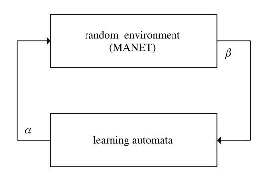
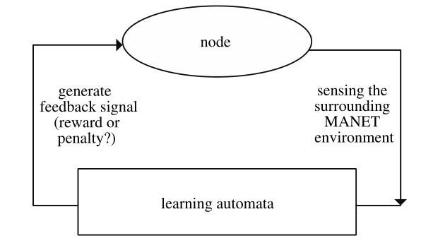

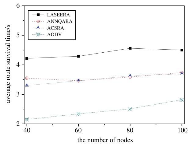
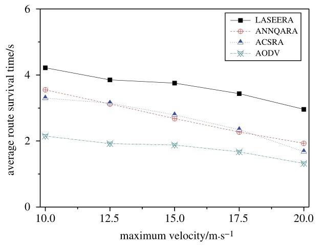


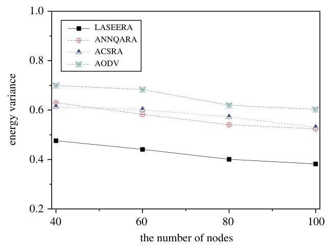
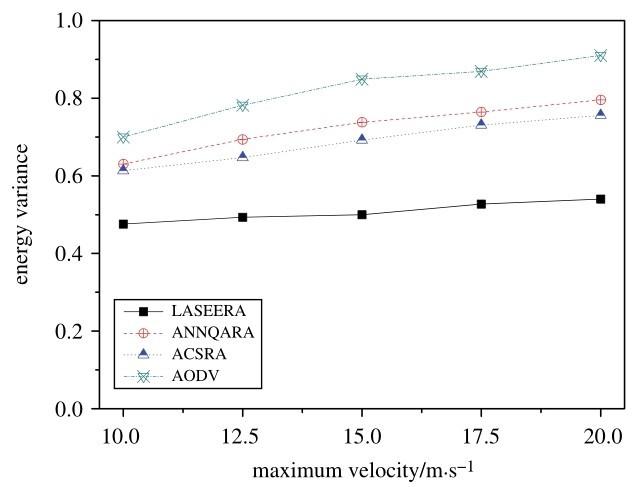
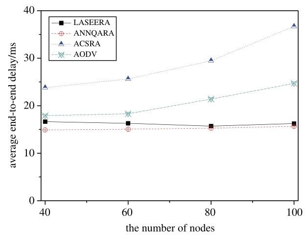
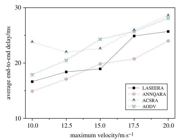
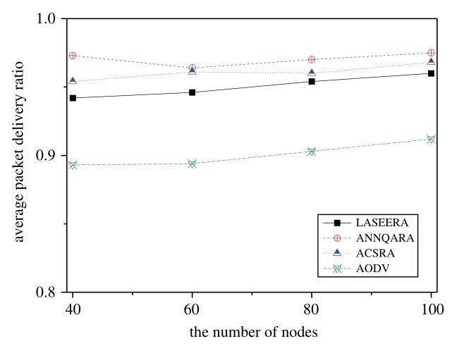

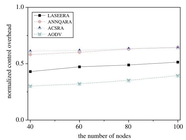
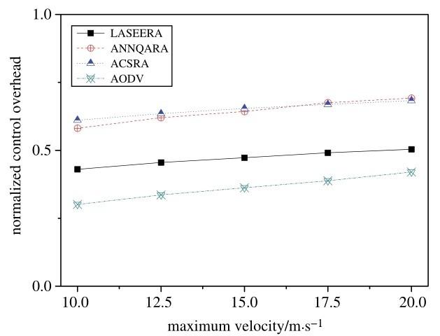
