The LNM Institute of Information Technology, Rupa Ki Nangal, Post-Sumel, viaJamdoli, Jaipur 302031, India
作者简介 About authors
Anirudh Agarwal[corresponding author]received his B Tech degree in 2014, and is pursuing his Ph D degree in Electronics & Communications Engineering from The LNM Institute of Information Technology (LNMⅡT), Jaipur, India He has been actively involved in the Indian Government project, “Mobile Broadband Service Support Over Cognitive Radio Networks”, funded by ITRA-MediaLab Asia, Ministry of Electronics&IT, Govt of India He has coauthored one book chapter and many papers in refereed journals and recognized conferences His research interests include mobile and wireless communication systems, with special emphasis on applied machine learning based quality of experience of CR users provisioning, spectrum occupancy modeling and dynamic spectrum access in CR networks
, E-mail:anirudh.agarwal@lnmiit.ac.in.
Aditya S Sengar received his B Tech degree in 2014, M Tech degree in 2016 and is pursuing his Ph D degree in Electronics&Communications Engineering from The LNM Institute of Information Technology(LNMⅡT), Jaipur, India He has co-authored many papers in refereed journals and recognized conferences His research interests include cognitive radio systems, device-to-device communication, 5G wireless networks
, E-mail:a.sengar.bkn@gmail.com.
Ranjan Gangopadhyay received his Ph D degree from IIT, Kharagpur He served as a professor and Head of the Department of E & ECE, IIT Kharagpur After superannuation (2006), he joined the G S Sanyal School of Telecommunication, IIT, Kharagpur as an Emeritus Professor and worked there for two years before joining The LNM Institute of Information Technology, Jaipur as a Distinguished Professor Prof Gangopadhyay has also served as a visiting professor in University of Parma(Italy), Scuola Superiore Sant’Anna, Pisa(Italy), British Telecom (UK), University of Ottawa, Chonbuk National University (South Korea)and Central Laboratory(Japan) His research interests include Photonics communication and wireless technology
, E-mail:ranjan iitkgp@yahoo.com.
Abstract
Spectrum occupancy information is necessary in a cognitive radio network (CRN) as it helps in modeling and predicting the spectrum availability for efficient dynamic spectrum access (DSA). However, in a CRN, it is difficult to ascertain a priori the pattern of the spectrum usage of the primary user due to its stochastic behavior. In this context, the spectrum occupancy prediction proves to be very useful in enhancing the quality of experience of the secondary user. This paper investigates the practical prowess of various time-series modeling approaches and the machine learning (ML) techniques for predicting spectrum occupancy, based on a spectrum measurement campaign conducted in Jaipur, Rajasthan, India. Moreover, the comparison analysis conducted between the above two approaches highlights the trade-off in terms of the respective performance depending upon the nature of the spectrum occupancy data. Nevertheless, prediction through ML-based recurrent neural network proves to perform reasonably well, thereby providing an accurate future spectrum occupancy information for DSA.
Anirudh Agarwal. Spectrum Occupancy Prediction for Realistic Traffic Scenarios: Time Series versus Learning-Based Models. [J], 2018, 3(2): 35-42 doi:10.1007/s41650-018-0013-6
Ⅰ. INTRODUCTION
The static nature of the contemporary spectrum allocationpolicy is the main cause of perceived spectrum scarcity today. The cognitive radio (CR) concepts are now mature enough to minimize spectrum under-utilization through opportunistic dynamic spectrum access (DSA). The CR transmission protocol allows a secondary user(SU)to smartly ac cess and utilize the resources of a primary user(PU)’s radio system and cease its transmission as soon as a PU is detected. In this process, the minimized use of spectrum sensing energy and better spectrum utilization are two significant criteria to be achieved for the CR users for efficient DSA. Moreover, prior information about the statistical behavior of the PU activity and its traffic load pattern are generally unknown in a realistic CR network. In this context, the available knowledge of PU spectrum occupancy is insufficient for DSA. To circumvent this limitation, certain spectrum prediction strategy at the SU level is highly desirable. Through a reliable prediction, the SU can efficiently access the available spectrum by using the future spectrum occupancy information, thus reducing the total number of spectrum-sensing events, and consequently, the required sensing energy. In fact, in this context, the authors in Ref. [1]have performed the descriptive predictability studies of radio spectrum state, quantified with respect to the entropy measurements and the Fano inequality. More recently, the upper and lower bounds on the predictability of various communication spectrum bands based on quantization levels of statistical entropies and regularity measure have been wellinvestigated in Ref. [2].
In the literature, stochastic models have been well appreciated for their ability to forecast time series in diverse fields, ranging from electricity price hike analysis to network traffic prediction[3] and spectrum occupancy modeling[4,5]. Meanwhile, machine learning(ML)has been proved to be very attractive in diverse applications related to CR operation, e. g. , optimized spectrum sensing, accurate PU load pattern prediction, and robust spectrum occupancy modeling[6]. Moreover, the potential applications of spectrum prediction also lie in spectrum mobility&spectrum sharing in 5G wireless networks, cognitive smart grid networks, and cognitive wireless sensor networks[7]. Few key quality features of ML algorithms rest in their adaptive ability to account for the dynamically varying statistics of wireless communication data as well as their efficacy in situations where the prior information of the incumbent distributions under consideration is unknown.
In the context of CR, for time-series modeling-based pre diction, an auto-regressive (AR) model for one-step spectral occupancy prediction of the GSM band was applied in Ref. [8], and was extended in Ref. [9]to compare the accuracy of the one-step ahead prediction with that of an n-step ahead prediction. In Ref. [10], a hybrid model comprising the auto regressive integrative moving average(ARIMA), along with seasonal ARIMA on the GSM band, was used. However, the ML-based approaches for CR applications include the multilayer perceptron technique, artificial neural networks(ANNs), and support vector machines (SVMs) that have been well investigated[11]. In Ref. [12], a functional link artificial neural network and multi-layer perceptron techniques have been used for spectrum prediction, but only in the Industrial, Scientific and Medical radio(ISM)band. In Ref. [13], Eltholth et al. used wavelet neural networks for spectrum prediction; however, 24 hr indoor data were considered and the focus was more toward hidden node problems rather than prediction. A detailed and comprehensive survey of spectrum prediction techniques has been rigorously carried out in Ref. [7]. The authors in Ref. [14]claimed that the“linear SVM(LSVM)”technique provides the best accuracy, among ANN, Gaussian SVM, and in fact the recurrent neural networks(RNNs), for PU traffic prediction in various known network data traffic scenarios. However, this observation may not be always true, e. g. , the case for any realistic PU traffic with inherent nonlinear behavior. Similarly, the time-series models may also prove to be useful in some of the traffic scenarios that exhibit a linear pattern. The above observations indicate a trade-off between the performance of time-series models and ML techniques depending upon the behavior of the input dataset. A comparative analysis of the predictive capability between the above methods is, therefore, required between time-series modeling and advanced ML techniques for a realistic CR-based spectrum environment, which has not been sufficiently conducted in the existing literature. Moreover, the accuracy of prediction models for different values of integration time has not been ana lyzed.
In this study, we have carried out spectrum occupancy prediction for the cases of stationary traffic of a TV band as well as non-stationary traffic in a cellular band, based on actual spectrum measurement data obtained after conducting a measurement campaign at Jaipur city, Rajasthan, India. The reason for considering two data traffics with different statistical behaviors is to compare the performance of one prediction scheme with that of the other, which depends on the nature of the input. This spectrum occupancy measurement data are used for prediction. Two widely used time-series models, i. e. , AR and ARIMA, are investigated and their performance results are further compared with those of two ML techniques: LSVM and RNN. In ML, LSVM is chosen to show that it is not the best prediction technique for all types of PU traffics. RNN is considered to be mathematically complex in implementation, but its robustness in realistic datasets and application novelty in the communication domain motivate us to analyze it against LSVM. The performance analysis of the prediction techniques is estimated on the basis of the meansquare error in the original and predicted spectrum occupancy data for different integration times.
The rest of the paper is organized as follows. Section Ⅱ discusses the system model and describes the data. A brief description of the time-series models and ML techniques is provided in sections Ⅲ and Ⅳ, respectively. The performance analysis and results are discussed in section V. Finally, section Ⅵ concludes the paper.
Ⅱ. SYSTEM MODEL AND METHODOLOGY
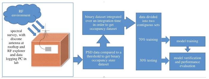
The system model shown in Fig.1 operates in two major phases: the spectrum occupancy measurement phase and the spectrum occupancy prediction phase. The measurement of spectrum occupancy is necessary in the contexts of both DSA and licensed shared access (LSA). The spectrum measurements considered in this study are conducted at LNMIIT, Jaipur, India(Latitude 26◦56’09. 8”N, Longitude 75◦55’27. 2”E). The major equipment includes a Sirio SD 1 300N omni-directional discone antenna and an RF explorerbased mini-spectrum analyzer. The spectrum analyzer configuration is indicated in Tab.1.
The measurements performed over a week are in terms of power spectrum density (PSD) over the frequency range, 150∼750 MHz in the TV band, and 850∼1 300 MHz in the cellular band(combination of GSM 900 uplink and downlink), recorded with a sweep time of 0.8 s. After digital switchover, a portion of the TV analog channels becomes entirely vacant due to the higher spectrum efficiency of digital TV[15], thereby suggesting an almost static PU traffic pattern in the TV band. However, the traffic load pattern of PUs in the cellular band is significantly dynamic and non-stationary, as indicated by the enormous number of mobile phone users accessing this GSM band.
Authors in Ref. [16]perform a robust spectrum prediction using real raw PSD data in different bands of interest. However, this study mainly focuses on spectrum occupancy prediction, so it is necessary to obtain the spectrum occupancy information from the available PSD data. For this purpose, a threshold is required over and above the noise fl oor, thereby classifying the PU traffic data into an occupied state(above the threshold) or an unoccupied state (below the threshold). In the present study, the most standard and well-investigated classical energy detection-based median filtering approach is adopted for threshold selection, which is detailed in Ref. [17]. As a result, the threshold is set as 4 dB above the noise fl oor for getting the appropriate and necessary spectrum occupancy information, also considering the effect of local outliers, in both the bands under consideration. The samples above the threshold represent the class of the occupied state of the PU and those below it correspond to that of the unoccupied state. This classification generates a binary spectrum occupancy state dataset, with“1”representing the occupied channel, while“0”representing the availability of the SU channel. To determine the spectrum occupancy for a particular duration, the binary data needs to be integrated over a time interval, i. e. , integration time(TI), which has typical values of 1, 5, 10, and 15 min over the entire observation interval. After the integration process, the values of the resultant spectrum occupancy dataset are normalized in the range of[0, 1].
The data are utilized as input for the purpose of prediction, to be used by either the time-series model or the ML technique. For prediction by either method, 70% of the data are used for training the model. Once the model is trained, it is used for testing the remaining 30%. The ratio of training data to testing data is chosen after sufficient iterative simulations with different training lengths(see section V).
Ⅲ. TIME-SERIES MODELS
We consider two time-series models: AR and ARIMA. The general expression for stationary time-series models is given by
where d is the order of differentiation, yt is the observed time series(t> 0), εt is an independent and identically distributed non-Gaussian sequence, is a back-shift operator, is the AR polynomial of order p, and is the“moving average polynomial”of order q.
An AR(p)model is defined as
where is the predicted series, φ j indicates the p model parameters, and εt denotes the innovation terms.
The auto-correlation function (ACF) and partial autocorrelation function (PACF) are important tools for timeseries model identification[18]. ACF ρk is defined as
where indicates the correlation coefficients at successive lags:
where N is the total number of samples in the time series yt.
In ACF, the term ρk describes the correlation between the observation at t=0 and that at t=k. It also considers the contribution from all intervening observations. In the case of PACF, the contributions from the intervening terms are removed.
In most real-life scenarios, the observed time series are difference stationary; that is, they can be made stationary through finite differentiation. The d term in ARIMA(p, d, q)represents the order of differentiation.
Ⅳ. ML TECHNIQUES
In this section, the two ML prediction techniques used in this study are briefl y described.
A. LSVM-Based Prediction
An SVM is a supervised ML algorithm that can be used for classification as well as regression. It classifies the data samples with a hyperplane, thereby obtaining a decision boundary that maximizes the distance between the support vectors. The support vectors include the data points closest to the hyperplane, whose position is based on that of a kernel. We use one variant of a kernel, i. e. , linear kernel. The ith training feature and response vectors are represented as , where Tiε{−1, 1}. The separating hyperplane is denoted as , where w is the weight vector, b is the bias, and is a slack variable vector whose single norm is the penalty term. The two classes separated by the hyperplane are given as
The following optimization problem for the SVM can be formed using a soft margin:
where C> 0 regularizes the weight of the penalty term and the margin maximization term [19].
We use the LIBSVM software tool, integrated and compiled in MATLAB[20]. The stopping criterion of the algorithm is achieved at the minimum tolerance value (0.0001 in this study).
B. RNNs
The major objective of an RNN is to optimally tap the computational power of a neural network by their ability to deal with the temporal dynamics of the data and to store the information for future use through recurrent connections. In this study, we use the most simplified model of RNNs, i. e. , Elman network(EN).
As shown in Fig.2, there are four layers in a simple Elmanbased RNN: input layer, hidden layer, context layer, and output layer. The context layer provides recurrent feedback to receive input from and then return the values to the hidden layer. At time t+1, the context layer receives a copy of the set of activations in the hidden layer at time t. In this feed-forward activation, the network is trained with the help of the backpropagation algorithm(BPA), thereby adjusting the weights. The background mathematics and further details on EN can be found in Ref. [21].
For the implementation purpose, the ML toolbox in MATLAB software has been used. The spectrum occupancy data with different integration times are individually put in the EN model. The number of neurons in the input layer, i. e. , the number of time samples of a channel taken at a time, is chosen as 4, with a single hidden layer having six neurons and an output layer with one neuron(see section V for details).
In this section, we discuss the governing metric and methodology used in analyzing the model structure in terms of selecting the training-testing ratio and various model parameters in time series as well as ML-based prediction techniques. There exist multitude of performance metrics for predictive analysis in the current literature[22]. However, for structural analysis of a predictive measure, we choose a modified form of mean absolute percentage error(MAPE), i. e. , mean absolute normalized error(MANE), which is defined as
where i denotes the prediction technique, N is the total number of simulation intervals, δpre(n)is the predicted spectrum occupancy of a primary channel at the nth simulation interval, and similarly, δorg(n)is the spectrum occupancy of a primary channel in the original data at the nth simulation interval.
It is similar to MAPE, except for the percentage term. The motivation behind using MANE is that for analyzing the model parameters, it is important to investigate the fractional estimate of the error with respect to the original data.
Consequently, the training length in Tab.2 and the set of model parameters are chosen corresponding to the minimum MANE value.
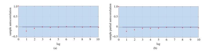
Figure 4
Differential ACF and PACF plots: (a)ACF plot for Yt; (b)PACF plot for Yt
A. Time-Series Model Order Estimation
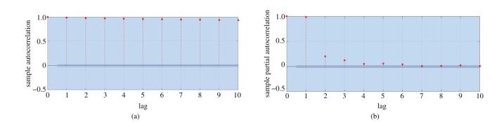
In this subsection, yt represents the time series representing the occupancy data of the TV band with 1-min integration time and Yt represents the time series obtained after finite differentiation of yt.
Fig.3(a)and(b)respectively represent the ACF and PACF plots for yt. As evident from these plots, a good estimate for the AR model order is 6. Fig.4(a)and(b)represent the ACF and PACF plots for Yt. The damped sinusoidal shape of both ACF and PACF indicates the adoption of an ARIMA model of a suitable order.
The actual model structure is determined through a comparison between a few candidate models based on the mean square error(MSE)performance, as indicated in Tabs. 3 and 4. The appropriate model orders for the remaining occupancy series for integration times of 5, 10, and 15 min are obtained similarly, and are thus, presented in Tab.5.
Table 3
Table 3 MANE for a few candidate time-series models in the TV band
In the RNN used in this study, only one hidden layer is found to be sufficient in the overall predictive modeling in terms of time as well as computational complexity. Although the choice of the input order, i. e. , 4, and the number of neurons in the hidden layer, i. e. , 8(or 10), is based on the lowest MANE value, as shown in Tab.6, we choose“6”as the optimal number of neurons in the hidden layer because the algorithm implementation due to an increment of 2(to make it 8) neurons in the hidden layer has been proved to be mathemat ically more complex as compared to a mere variation in the system performance due to a difference of just 0.001 in the value of MANE.
Table 6
Table 6 MANE for different numbers of neurons in different RNN layers
After appropriate model structure selection through MANE, the resulting spectrum occupancy prediction accuracy of a particular prediction technique is evaluated on the basis of the MSEi in predicting the spectrum occupancy of a primary channel for the next time duration depending upon different integration times—1, 5, 10, and 15 min, which is given as
The variables in the above equation are the same as those described in section V.
For prediction analysis, 70% of the spectrum occupancy data are used for training, while the rest are used for testing the trained model.
Tab.7 compares the accuracies of all considered prediction schemes for different integration times in the TV band. The table shows that, for higher integration time, MSEi increases in all cases. This is attributed to the fact that more data for training result in better prediction performance. When the integration time increases, the number of data points required for training the prediction model reduces, thereby providing less information to estimate the model parameters. In addition, the accuracy of time-series models tends to nearly approach to that of the ML techniques. This is supported by the fact that in the TV band, the traffic pattern is stationary, leading to some linearity in the dataset, where the time-series models can work quite efficiently. However, the AR model appears to perform slightly better in terms of MSEi than the ARIMA model. But at the cost of increased complexity owing to higher model orders.
Similarly, Tab.8 presents a comparison of the accuracies of the prediction techniques for different integration times in the cellular band. Even in this case, MSEi increases with respect to the integration time, and the reason for which has already been explained above. However, as the cellular band data traffic is non-stationary in nature with several irregularities, the ML techniques outperform the time-series models in terms of prediction accuracy. However, among the ML techniques used, RNN is observed to be more accurate than LSVM. As specified in part B of section Ⅳ, RNN has a feedback feature, according to which the predicted results are also used as its input, thereby improving its predictability. In LSVM, a linear kernel is used, which performs best where difficult decisions are to be taken, i. e. , whether 0 or 1, but in case of real-time spectrum occupancy prediction, soft decisions are required, where the performance of LSVM generally degrades.
Table 7
Table 7 Comparison of the prediction techniques’accuracies for different integration times in the TV band
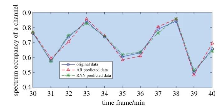
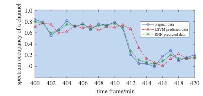
Figs. 5 and 6 depict the realistic spectrum occupancy data for 1-min integration time along with the predicted spectrum occupancy of a primary channel for the next minute, through various prediction techniques in the TV band and the cellular band, respectively. The results are presented for a PU channel in a particular time span of 10 or 20 min depending upon the sufficiency of the number of data points to be shown in a band. As indicated by Tab.7, the predicted results achieved by the two corresponding best prediction techniques, i. e. , one that is a better time-series model and the other that is a better ML prediction technique, are shown in Fig.5. It can be seen that the predicted outcome of AR is approximately comparable with that of RNN. In Fig.6, time-series model-based prediction has not been taken into consideration because their accuracy is not really at par with that of the ML techniques which can be observed in Tab.8. It is found that RNN-based spectrum occupancy prediction shows better accuracy when compared to LSVM.
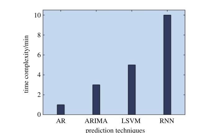
Furthermore, the time complexity of the considered prediction techniques is analyzed in Fig.7. In this paper, time complexity is defined in terms of the time taken by an algorithm to complete its single iteration, and it is found that the ML techniques are more complex than the time-series models due to their simplicity in implementation, unlike ML techniques.
Figure 7
Time complexity analysis of different prediction techniques
Ⅶ. CONCLUSION
In this study, the importance of real-time spectrum occupancy prediction is highlighted in the context of CR for efficient DSA by using time-series models and ML techniques. Both time-series modeling and ML-based prediction are found to be reasonably good in predicting the spectrum occupancy. However, there is a trade-off between the two, i. e. , when there is a seasonal or periodical trend in the dataset, the time-series models perform well in predicting the spectrum occupancy and that too with less computational complexity, while in case of data irregularities, ML techniques are more accurate. Furthermore, AR models in time-series modeling and RNN-based prediction in ML techniques perform better than their respective counterpart models. Among all the prediction techniques considered, it can be concluded that in case of real-time scenarios, the deep belief neural network-based RNN generally exhibits the highest accuracy, but is at the cost of increased implementation complexity.
The authors have declared that no competing interests exist.
Application of artificial neural network and support vector regression in cognitive radio networks for RF power prediction using compact differential evolution algorithm
[C]// IEEE Federated Conference on Computer Science and Information Systems(FedCSIS),L´odz, 2015: 55-66.
On the limits of predictability in realworld radio spectrum state dynamics: from entropy theory to 5G spectrum sharing
1
2015
... The static nature of the contemporary spectrum allocationpolicy is the main cause of perceived spectrum scarcity today. The cognitive radio (CR) concepts are now mature enough to minimize spectrum under-utilization through opportunistic dynamic spectrum access (DSA). The CR transmission protocol allows a secondary user(SU)to smartly ac cess and utilize the resources of a primary user(PU)’s radio system and cease its transmission as soon as a PU is detected. In this process, the minimized use of spectrum sensing energy and better spectrum utilization are two significant criteria to be achieved for the CR users for efficient DSA. Moreover, prior information about the statistical behavior of the PU activity and its traffic load pattern are generally unknown in a realistic CR network. In this context, the available knowledge of PU spectrum occupancy is insufficient for DSA. To circumvent this limitation, certain spectrum prediction strategy at the SU level is highly desirable. Through a reliable prediction, the SU can efficiently access the available spectrum by using the future spectrum occupancy information, thus reducing the total number of spectrum-sensing events, and consequently, the required sensing energy. In fact, in this context, the authors in Ref. [1]have performed the descriptive predictability studies of radio spectrum state, quantified with respect to the entropy measurements and the Fano inequality. More recently, the upper and lower bounds on the predictability of various communication spectrum bands based on quantization levels of statistical entropies and regularity measure have been wellinvestigated in Ref. [2]. ...
Predictability analysis of spectrum state evolution: performance bounds and real-world data analytics
1
2017
... The static nature of the contemporary spectrum allocationpolicy is the main cause of perceived spectrum scarcity today. The cognitive radio (CR) concepts are now mature enough to minimize spectrum under-utilization through opportunistic dynamic spectrum access (DSA). The CR transmission protocol allows a secondary user(SU)to smartly ac cess and utilize the resources of a primary user(PU)’s radio system and cease its transmission as soon as a PU is detected. In this process, the minimized use of spectrum sensing energy and better spectrum utilization are two significant criteria to be achieved for the CR users for efficient DSA. Moreover, prior information about the statistical behavior of the PU activity and its traffic load pattern are generally unknown in a realistic CR network. In this context, the available knowledge of PU spectrum occupancy is insufficient for DSA. To circumvent this limitation, certain spectrum prediction strategy at the SU level is highly desirable. Through a reliable prediction, the SU can efficiently access the available spectrum by using the future spectrum occupancy information, thus reducing the total number of spectrum-sensing events, and consequently, the required sensing energy. In fact, in this context, the authors in Ref. [1]have performed the descriptive predictability studies of radio spectrum state, quantified with respect to the entropy measurements and the Fano inequality. More recently, the upper and lower bounds on the predictability of various communication spectrum bands based on quantization levels of statistical entropies and regularity measure have been wellinvestigated in Ref. [2]. ...
Network traffic prediction and result analysis based on seasonal ARIMA and correlation coefficient
1
2010
... In the literature, stochastic models have been well appreciated for their ability to forecast time series in diverse fields, ranging from electricity price hike analysis to network traffic prediction[3] and spectrum occupancy modeling[4,5]. Meanwhile, machine learning(ML)has been proved to be very attractive in diverse applications related to CR operation, e. g. , optimized spectrum sensing, accurate PU load pattern prediction, and robust spectrum occupancy modeling[6]. Moreover, the potential applications of spectrum prediction also lie in spectrum mobility&spectrum sharing in 5G wireless networks, cognitive smart grid networks, and cognitive wireless sensor networks[7]. Few key quality features of ML algorithms rest in their adaptive ability to account for the dynamically varying statistics of wireless communication data as well as their efficacy in situations where the prior information of the incumbent distributions under consideration is unknown. ...
Spectrum occupancy statistics and time series models for cognitive radio
2
2011
... In the literature, stochastic models have been well appreciated for their ability to forecast time series in diverse fields, ranging from electricity price hike analysis to network traffic prediction[3] and spectrum occupancy modeling[4,5]. Meanwhile, machine learning(ML)has been proved to be very attractive in diverse applications related to CR operation, e. g. , optimized spectrum sensing, accurate PU load pattern prediction, and robust spectrum occupancy modeling[6]. Moreover, the potential applications of spectrum prediction also lie in spectrum mobility&spectrum sharing in 5G wireless networks, cognitive smart grid networks, and cognitive wireless sensor networks[7]. Few key quality features of ML algorithms rest in their adaptive ability to account for the dynamically varying statistics of wireless communication data as well as their efficacy in situations where the prior information of the incumbent distributions under consideration is unknown. ...
... The actual model structure is determined through a comparison between a few candidate models based on the mean square error(MSE)performance, as indicated in Tabs. 3 and 4. The appropriate model orders for the remaining occupancy series for integration times of 5, 10, and 15 min are obtained similarly, and are thus, presented in Tab.5. ...
Lessons learned from an extensive spectrum occupancy measurement campaign and a stochastic duty cycle model
1
2010
... In the literature, stochastic models have been well appreciated for their ability to forecast time series in diverse fields, ranging from electricity price hike analysis to network traffic prediction[3] and spectrum occupancy modeling[4,5]. Meanwhile, machine learning(ML)has been proved to be very attractive in diverse applications related to CR operation, e. g. , optimized spectrum sensing, accurate PU load pattern prediction, and robust spectrum occupancy modeling[6]. Moreover, the potential applications of spectrum prediction also lie in spectrum mobility&spectrum sharing in 5G wireless networks, cognitive smart grid networks, and cognitive wireless sensor networks[7]. Few key quality features of ML algorithms rest in their adaptive ability to account for the dynamically varying statistics of wireless communication data as well as their efficacy in situations where the prior information of the incumbent distributions under consideration is unknown. ...
Analysis of spectrum occupancy using machine learning algorithms
1
2016
... In the literature, stochastic models have been well appreciated for their ability to forecast time series in diverse fields, ranging from electricity price hike analysis to network traffic prediction[3] and spectrum occupancy modeling[4,5]. Meanwhile, machine learning(ML)has been proved to be very attractive in diverse applications related to CR operation, e. g. , optimized spectrum sensing, accurate PU load pattern prediction, and robust spectrum occupancy modeling[6]. Moreover, the potential applications of spectrum prediction also lie in spectrum mobility&spectrum sharing in 5G wireless networks, cognitive smart grid networks, and cognitive wireless sensor networks[7]. Few key quality features of ML algorithms rest in their adaptive ability to account for the dynamically varying statistics of wireless communication data as well as their efficacy in situations where the prior information of the incumbent distributions under consideration is unknown. ...
Spectrum inference in cognitive radio networks: algorithms and applications
2
2017
... In the literature, stochastic models have been well appreciated for their ability to forecast time series in diverse fields, ranging from electricity price hike analysis to network traffic prediction[3] and spectrum occupancy modeling[4,5]. Meanwhile, machine learning(ML)has been proved to be very attractive in diverse applications related to CR operation, e. g. , optimized spectrum sensing, accurate PU load pattern prediction, and robust spectrum occupancy modeling[6]. Moreover, the potential applications of spectrum prediction also lie in spectrum mobility&spectrum sharing in 5G wireless networks, cognitive smart grid networks, and cognitive wireless sensor networks[7]. Few key quality features of ML algorithms rest in their adaptive ability to account for the dynamically varying statistics of wireless communication data as well as their efficacy in situations where the prior information of the incumbent distributions under consideration is unknown. ...
... In the context of CR, for time-series modeling-based pre diction, an auto-regressive (AR) model for one-step spectral occupancy prediction of the GSM band was applied in Ref. [8], and was extended in Ref. [9]to compare the accuracy of the one-step ahead prediction with that of an n-step ahead prediction. In Ref. [10], a hybrid model comprising the auto regressive integrative moving average(ARIMA), along with seasonal ARIMA on the GSM band, was used. However, the ML-based approaches for CR applications include the multilayer perceptron technique, artificial neural networks(ANNs), and support vector machines (SVMs) that have been well investigated[11]. In Ref. [12], a functional link artificial neural network and multi-layer perceptron techniques have been used for spectrum prediction, but only in the Industrial, Scientific and Medical radio(ISM)band. In Ref. [13], Eltholth et al. used wavelet neural networks for spectrum prediction; however, 24 hr indoor data were considered and the focus was more toward hidden node problems rather than prediction. A detailed and comprehensive survey of spectrum prediction techniques has been rigorously carried out in Ref. [7]. The authors in Ref. [14]claimed that the“linear SVM(LSVM)”technique provides the best accuracy, among ANN, Gaussian SVM, and in fact the recurrent neural networks(RNNs), for PU traffic prediction in various known network data traffic scenarios. However, this observation may not be always true, e. g. , the case for any realistic PU traffic with inherent nonlinear behavior. Similarly, the time-series models may also prove to be useful in some of the traffic scenarios that exhibit a linear pattern. The above observations indicate a trade-off between the performance of time-series models and ML techniques depending upon the behavior of the input dataset. A comparative analysis of the predictive capability between the above methods is, therefore, required between time-series modeling and advanced ML techniques for a realistic CR-based spectrum environment, which has not been sufficiently conducted in the existing literature. Moreover, the accuracy of prediction models for different values of integration time has not been ana lyzed. ...
Binary time series approach to spectrum prediction for cognitive radio
1
2007
... In the context of CR, for time-series modeling-based pre diction, an auto-regressive (AR) model for one-step spectral occupancy prediction of the GSM band was applied in Ref. [8], and was extended in Ref. [9]to compare the accuracy of the one-step ahead prediction with that of an n-step ahead prediction. In Ref. [10], a hybrid model comprising the auto regressive integrative moving average(ARIMA), along with seasonal ARIMA on the GSM band, was used. However, the ML-based approaches for CR applications include the multilayer perceptron technique, artificial neural networks(ANNs), and support vector machines (SVMs) that have been well investigated[11]. In Ref. [12], a functional link artificial neural network and multi-layer perceptron techniques have been used for spectrum prediction, but only in the Industrial, Scientific and Medical radio(ISM)band. In Ref. [13], Eltholth et al. used wavelet neural networks for spectrum prediction; however, 24 hr indoor data were considered and the focus was more toward hidden node problems rather than prediction. A detailed and comprehensive survey of spectrum prediction techniques has been rigorously carried out in Ref. [7]. The authors in Ref. [14]claimed that the“linear SVM(LSVM)”technique provides the best accuracy, among ANN, Gaussian SVM, and in fact the recurrent neural networks(RNNs), for PU traffic prediction in various known network data traffic scenarios. However, this observation may not be always true, e. g. , the case for any realistic PU traffic with inherent nonlinear behavior. Similarly, the time-series models may also prove to be useful in some of the traffic scenarios that exhibit a linear pattern. The above observations indicate a trade-off between the performance of time-series models and ML techniques depending upon the behavior of the input dataset. A comparative analysis of the predictive capability between the above methods is, therefore, required between time-series modeling and advanced ML techniques for a realistic CR-based spectrum environment, which has not been sufficiently conducted in the existing literature. Moreover, the accuracy of prediction models for different values of integration time has not been ana lyzed. ...
Predicting radio resource availability in cognitive radio—an experimental examination
1
2008
... In the context of CR, for time-series modeling-based pre diction, an auto-regressive (AR) model for one-step spectral occupancy prediction of the GSM band was applied in Ref. [8], and was extended in Ref. [9]to compare the accuracy of the one-step ahead prediction with that of an n-step ahead prediction. In Ref. [10], a hybrid model comprising the auto regressive integrative moving average(ARIMA), along with seasonal ARIMA on the GSM band, was used. However, the ML-based approaches for CR applications include the multilayer perceptron technique, artificial neural networks(ANNs), and support vector machines (SVMs) that have been well investigated[11]. In Ref. [12], a functional link artificial neural network and multi-layer perceptron techniques have been used for spectrum prediction, but only in the Industrial, Scientific and Medical radio(ISM)band. In Ref. [13], Eltholth et al. used wavelet neural networks for spectrum prediction; however, 24 hr indoor data were considered and the focus was more toward hidden node problems rather than prediction. A detailed and comprehensive survey of spectrum prediction techniques has been rigorously carried out in Ref. [7]. The authors in Ref. [14]claimed that the“linear SVM(LSVM)”technique provides the best accuracy, among ANN, Gaussian SVM, and in fact the recurrent neural networks(RNNs), for PU traffic prediction in various known network data traffic scenarios. However, this observation may not be always true, e. g. , the case for any realistic PU traffic with inherent nonlinear behavior. Similarly, the time-series models may also prove to be useful in some of the traffic scenarios that exhibit a linear pattern. The above observations indicate a trade-off between the performance of time-series models and ML techniques depending upon the behavior of the input dataset. A comparative analysis of the predictive capability between the above methods is, therefore, required between time-series modeling and advanced ML techniques for a realistic CR-based spectrum environment, which has not been sufficiently conducted in the existing literature. Moreover, the accuracy of prediction models for different values of integration time has not been ana lyzed. ...
Modeling of GSM spectrum based on seasonal arima model
1
2014
... In the context of CR, for time-series modeling-based pre diction, an auto-regressive (AR) model for one-step spectral occupancy prediction of the GSM band was applied in Ref. [8], and was extended in Ref. [9]to compare the accuracy of the one-step ahead prediction with that of an n-step ahead prediction. In Ref. [10], a hybrid model comprising the auto regressive integrative moving average(ARIMA), along with seasonal ARIMA on the GSM band, was used. However, the ML-based approaches for CR applications include the multilayer perceptron technique, artificial neural networks(ANNs), and support vector machines (SVMs) that have been well investigated[11]. In Ref. [12], a functional link artificial neural network and multi-layer perceptron techniques have been used for spectrum prediction, but only in the Industrial, Scientific and Medical radio(ISM)band. In Ref. [13], Eltholth et al. used wavelet neural networks for spectrum prediction; however, 24 hr indoor data were considered and the focus was more toward hidden node problems rather than prediction. A detailed and comprehensive survey of spectrum prediction techniques has been rigorously carried out in Ref. [7]. The authors in Ref. [14]claimed that the“linear SVM(LSVM)”technique provides the best accuracy, among ANN, Gaussian SVM, and in fact the recurrent neural networks(RNNs), for PU traffic prediction in various known network data traffic scenarios. However, this observation may not be always true, e. g. , the case for any realistic PU traffic with inherent nonlinear behavior. Similarly, the time-series models may also prove to be useful in some of the traffic scenarios that exhibit a linear pattern. The above observations indicate a trade-off between the performance of time-series models and ML techniques depending upon the behavior of the input dataset. A comparative analysis of the predictive capability between the above methods is, therefore, required between time-series modeling and advanced ML techniques for a realistic CR-based spectrum environment, which has not been sufficiently conducted in the existing literature. Moreover, the accuracy of prediction models for different values of integration time has not been ana lyzed. ...
Application of artificial neural network and support vector regression in cognitive radio networks for RF power prediction using compact differential evolution algorithm
1
2015
... In the context of CR, for time-series modeling-based pre diction, an auto-regressive (AR) model for one-step spectral occupancy prediction of the GSM band was applied in Ref. [8], and was extended in Ref. [9]to compare the accuracy of the one-step ahead prediction with that of an n-step ahead prediction. In Ref. [10], a hybrid model comprising the auto regressive integrative moving average(ARIMA), along with seasonal ARIMA on the GSM band, was used. However, the ML-based approaches for CR applications include the multilayer perceptron technique, artificial neural networks(ANNs), and support vector machines (SVMs) that have been well investigated[11]. In Ref. [12], a functional link artificial neural network and multi-layer perceptron techniques have been used for spectrum prediction, but only in the Industrial, Scientific and Medical radio(ISM)band. In Ref. [13], Eltholth et al. used wavelet neural networks for spectrum prediction; however, 24 hr indoor data were considered and the focus was more toward hidden node problems rather than prediction. A detailed and comprehensive survey of spectrum prediction techniques has been rigorously carried out in Ref. [7]. The authors in Ref. [14]claimed that the“linear SVM(LSVM)”technique provides the best accuracy, among ANN, Gaussian SVM, and in fact the recurrent neural networks(RNNs), for PU traffic prediction in various known network data traffic scenarios. However, this observation may not be always true, e. g. , the case for any realistic PU traffic with inherent nonlinear behavior. Similarly, the time-series models may also prove to be useful in some of the traffic scenarios that exhibit a linear pattern. The above observations indicate a trade-off between the performance of time-series models and ML techniques depending upon the behavior of the input dataset. A comparative analysis of the predictive capability between the above methods is, therefore, required between time-series modeling and advanced ML techniques for a realistic CR-based spectrum environment, which has not been sufficiently conducted in the existing literature. Moreover, the accuracy of prediction models for different values of integration time has not been ana lyzed. ...
Spectrum occupancy prediction based on functional link artificial neural network(FLANN)in ISM band
1
2016
... In the context of CR, for time-series modeling-based pre diction, an auto-regressive (AR) model for one-step spectral occupancy prediction of the GSM band was applied in Ref. [8], and was extended in Ref. [9]to compare the accuracy of the one-step ahead prediction with that of an n-step ahead prediction. In Ref. [10], a hybrid model comprising the auto regressive integrative moving average(ARIMA), along with seasonal ARIMA on the GSM band, was used. However, the ML-based approaches for CR applications include the multilayer perceptron technique, artificial neural networks(ANNs), and support vector machines (SVMs) that have been well investigated[11]. In Ref. [12], a functional link artificial neural network and multi-layer perceptron techniques have been used for spectrum prediction, but only in the Industrial, Scientific and Medical radio(ISM)band. In Ref. [13], Eltholth et al. used wavelet neural networks for spectrum prediction; however, 24 hr indoor data were considered and the focus was more toward hidden node problems rather than prediction. A detailed and comprehensive survey of spectrum prediction techniques has been rigorously carried out in Ref. [7]. The authors in Ref. [14]claimed that the“linear SVM(LSVM)”technique provides the best accuracy, among ANN, Gaussian SVM, and in fact the recurrent neural networks(RNNs), for PU traffic prediction in various known network data traffic scenarios. However, this observation may not be always true, e. g. , the case for any realistic PU traffic with inherent nonlinear behavior. Similarly, the time-series models may also prove to be useful in some of the traffic scenarios that exhibit a linear pattern. The above observations indicate a trade-off between the performance of time-series models and ML techniques depending upon the behavior of the input dataset. A comparative analysis of the predictive capability between the above methods is, therefore, required between time-series modeling and advanced ML techniques for a realistic CR-based spectrum environment, which has not been sufficiently conducted in the existing literature. Moreover, the accuracy of prediction models for different values of integration time has not been ana lyzed. ...
Spectrum prediction in cognitive radio systems using a wavelet neural network
1
2016
... In the context of CR, for time-series modeling-based pre diction, an auto-regressive (AR) model for one-step spectral occupancy prediction of the GSM band was applied in Ref. [8], and was extended in Ref. [9]to compare the accuracy of the one-step ahead prediction with that of an n-step ahead prediction. In Ref. [10], a hybrid model comprising the auto regressive integrative moving average(ARIMA), along with seasonal ARIMA on the GSM band, was used. However, the ML-based approaches for CR applications include the multilayer perceptron technique, artificial neural networks(ANNs), and support vector machines (SVMs) that have been well investigated[11]. In Ref. [12], a functional link artificial neural network and multi-layer perceptron techniques have been used for spectrum prediction, but only in the Industrial, Scientific and Medical radio(ISM)band. In Ref. [13], Eltholth et al. used wavelet neural networks for spectrum prediction; however, 24 hr indoor data were considered and the focus was more toward hidden node problems rather than prediction. A detailed and comprehensive survey of spectrum prediction techniques has been rigorously carried out in Ref. [7]. The authors in Ref. [14]claimed that the“linear SVM(LSVM)”technique provides the best accuracy, among ANN, Gaussian SVM, and in fact the recurrent neural networks(RNNs), for PU traffic prediction in various known network data traffic scenarios. However, this observation may not be always true, e. g. , the case for any realistic PU traffic with inherent nonlinear behavior. Similarly, the time-series models may also prove to be useful in some of the traffic scenarios that exhibit a linear pattern. The above observations indicate a trade-off between the performance of time-series models and ML techniques depending upon the behavior of the input dataset. A comparative analysis of the predictive capability between the above methods is, therefore, required between time-series modeling and advanced ML techniques for a realistic CR-based spectrum environment, which has not been sufficiently conducted in the existing literature. Moreover, the accuracy of prediction models for different values of integration time has not been ana lyzed. ...
Learning based primary user activity prediction in cognitive radio networks for efficient dynamic spectrum access
1
2016
... In the context of CR, for time-series modeling-based pre diction, an auto-regressive (AR) model for one-step spectral occupancy prediction of the GSM band was applied in Ref. [8], and was extended in Ref. [9]to compare the accuracy of the one-step ahead prediction with that of an n-step ahead prediction. In Ref. [10], a hybrid model comprising the auto regressive integrative moving average(ARIMA), along with seasonal ARIMA on the GSM band, was used. However, the ML-based approaches for CR applications include the multilayer perceptron technique, artificial neural networks(ANNs), and support vector machines (SVMs) that have been well investigated[11]. In Ref. [12], a functional link artificial neural network and multi-layer perceptron techniques have been used for spectrum prediction, but only in the Industrial, Scientific and Medical radio(ISM)band. In Ref. [13], Eltholth et al. used wavelet neural networks for spectrum prediction; however, 24 hr indoor data were considered and the focus was more toward hidden node problems rather than prediction. A detailed and comprehensive survey of spectrum prediction techniques has been rigorously carried out in Ref. [7]. The authors in Ref. [14]claimed that the“linear SVM(LSVM)”technique provides the best accuracy, among ANN, Gaussian SVM, and in fact the recurrent neural networks(RNNs), for PU traffic prediction in various known network data traffic scenarios. However, this observation may not be always true, e. g. , the case for any realistic PU traffic with inherent nonlinear behavior. Similarly, the time-series models may also prove to be useful in some of the traffic scenarios that exhibit a linear pattern. The above observations indicate a trade-off between the performance of time-series models and ML techniques depending upon the behavior of the input dataset. A comparative analysis of the predictive capability between the above methods is, therefore, required between time-series modeling and advanced ML techniques for a realistic CR-based spectrum environment, which has not been sufficiently conducted in the existing literature. Moreover, the accuracy of prediction models for different values of integration time has not been ana lyzed. ...
A survey of cognitive radio access to TV White Spaces
1
2010
... The measurements performed over a week are in terms of power spectrum density (PSD) over the frequency range, 150∼750 MHz in the TV band, and 850∼1 300 MHz in the cellular band(combination of GSM 900 uplink and downlink), recorded with a sweep time of 0.8 s. After digital switchover, a portion of the TV analog channels becomes entirely vacant due to the higher spectrum efficiency of digital TV[15], thereby suggesting an almost static PU traffic pattern in the TV band. However, the traffic load pattern of PUs in the cellular band is significantly dynamic and non-stationary, as indicated by the enormous number of mobile phone users accessing this GSM band. ...
Robust online spectrum prediction with incomplete and corrupted historical observations
1
2017
... Authors in Ref. [16]perform a robust spectrum prediction using real raw PSD data in different bands of interest. However, this study mainly focuses on spectrum occupancy prediction, so it is necessary to obtain the spectrum occupancy information from the available PSD data. For this purpose, a threshold is required over and above the noise fl oor, thereby classifying the PU traffic data into an occupied state(above the threshold) or an unoccupied state (below the threshold). In the present study, the most standard and well-investigated classical energy detection-based median filtering approach is adopted for threshold selection, which is detailed in Ref. [17]. As a result, the threshold is set as 4 dB above the noise fl oor for getting the appropriate and necessary spectrum occupancy information, also considering the effect of local outliers, in both the bands under consideration. The samples above the threshold represent the class of the occupied state of the PU and those below it correspond to that of the unoccupied state. This classification generates a binary spectrum occupancy state dataset, with“1”representing the occupied channel, while“0”representing the availability of the SU channel. To determine the spectrum occupancy for a particular duration, the binary data needs to be integrated over a time interval, i. e. , integration time(TI), which has typical values of 1, 5, 10, and 15 min over the entire observation interval. After the integration process, the values of the resultant spectrum occupancy dataset are normalized in the range of[0, 1]. ...
Spectrum occupancy measurements and analysis in Beijing
1
2013
... Authors in Ref. [16]perform a robust spectrum prediction using real raw PSD data in different bands of interest. However, this study mainly focuses on spectrum occupancy prediction, so it is necessary to obtain the spectrum occupancy information from the available PSD data. For this purpose, a threshold is required over and above the noise fl oor, thereby classifying the PU traffic data into an occupied state(above the threshold) or an unoccupied state (below the threshold). In the present study, the most standard and well-investigated classical energy detection-based median filtering approach is adopted for threshold selection, which is detailed in Ref. [17]. As a result, the threshold is set as 4 dB above the noise fl oor for getting the appropriate and necessary spectrum occupancy information, also considering the effect of local outliers, in both the bands under consideration. The samples above the threshold represent the class of the occupied state of the PU and those below it correspond to that of the unoccupied state. This classification generates a binary spectrum occupancy state dataset, with“1”representing the occupied channel, while“0”representing the availability of the SU channel. To determine the spectrum occupancy for a particular duration, the binary data needs to be integrated over a time interval, i. e. , integration time(TI), which has typical values of 1, 5, 10, and 15 min over the entire observation interval. After the integration process, the values of the resultant spectrum occupancy dataset are normalized in the range of[0, 1]. ...
Time Series Analysis: Forecasting and Control
1
2015
... The auto-correlation function (ACF) and partial autocorrelation function (PACF) are important tools for timeseries model identification[18]. ACF ρk is defined as ...
A tutorial on support vector machines for pattern recognition
1
1998
... where C> 0 regularizes the weight of the penalty term and the margin maximization term [19]. ...
Libsvm: a library for support vector machines
1
2011
... We use the LIBSVM software tool, integrated and compiled in MATLAB[20]. The stopping criterion of the algorithm is achieved at the minimum tolerance value (0.0001 in this study). ...
Elman neural networks for characterizing voids in welded strips: a study
1
2012
... As shown in Fig.2, there are four layers in a simple Elmanbased RNN: input layer, hidden layer, context layer, and output layer. The context layer provides recurrent feedback to receive input from and then return the values to the hidden layer. At time t+1, the context layer receives a copy of the set of activations in the hidden layer at time t. In this feed-forward activation, the network is trained with the help of the backpropagation algorithm(BPA), thereby adjusting the weights. The background mathematics and further details on EN can be found in Ref. [21]. ...
Error measures for generalizing about forecasting methods: Empirical comparisons
1
1992
... In this section, we discuss the governing metric and methodology used in analyzing the model structure in terms of selecting the training-testing ratio and various model parameters in time series as well as ML-based prediction techniques. There exist multitude of performance metrics for predictive analysis in the current literature[22]. However, for structural analysis of a predictive measure, we choose a modified form of mean absolute percentage error(MAPE), i. e. , mean absolute normalized error(MANE), which is defined as ...


